
Christopher Paul shared his EDN technical article on third order low pass filter with a single operational amplifier.
A number of years ago, I posted an article and spreadsheet on EDN that enables the design of 2nd and 3rd order Sallen-Key low pass filters given the poles of their filter characteristics. The user enters the values of the capacitors and of those resistors which set the DC gain of the single op amp employed by the filter. After specifying the tolerances of all passive components and selecting an “E” series of resistor values (E-12, E-24, E-48, E-96 or E-192), the spreadsheet calculates the nearest commercially available values of the unspecified resistors. It also calculates the root of the sum of the squares of the sensitivity of the magnitude of the filter response to all passive components. It does this at a user-specified frequency (recommended to be at resonance, where sensitivity is the highest.)
One limitation of this procedure is that it relies on the user to specify different combinations of component values in search of solutions with ever lower sensitivities. This is tedious, and there is no guarantee that the lowest sensitivity solution will ever be found. This article discusses an approach and provides an executable program that remedies this situation. Given filter poles and capacitor and resistor E-series values and range limits, the program tests all possible component combinations and identifies the solutions with the lowest (and what the heck, the highest) aggregate component value sensitivities.
Why all this effort for third order filters?
Well, why not? If you can add an extra pole’s worth of attenuation without having to add an op amp, why wouldn’t you at least consider this? But there’s an even better reason – avoiding stopband leakage (see the section of the same name in the article cited above.) Briefly, as op amp open loop gain falls with higher frequencies in a second order Sallen Key section, its output impedance rises. The section’s input signal is capacitively coupled to the op amp output. The result is that higher frequency stopband rejection is a lot worse than intended. A third order design remedies this by inserting an R-C section (whose capacitor is grounded) between the input and output. By attenuating the portion of input signal which reaches the filter capacitor connected to the output, stopband rejection is significantly improved. The effect of the op amp’s rising output impedance can is accordingly rendered negligible.
Getting down to it
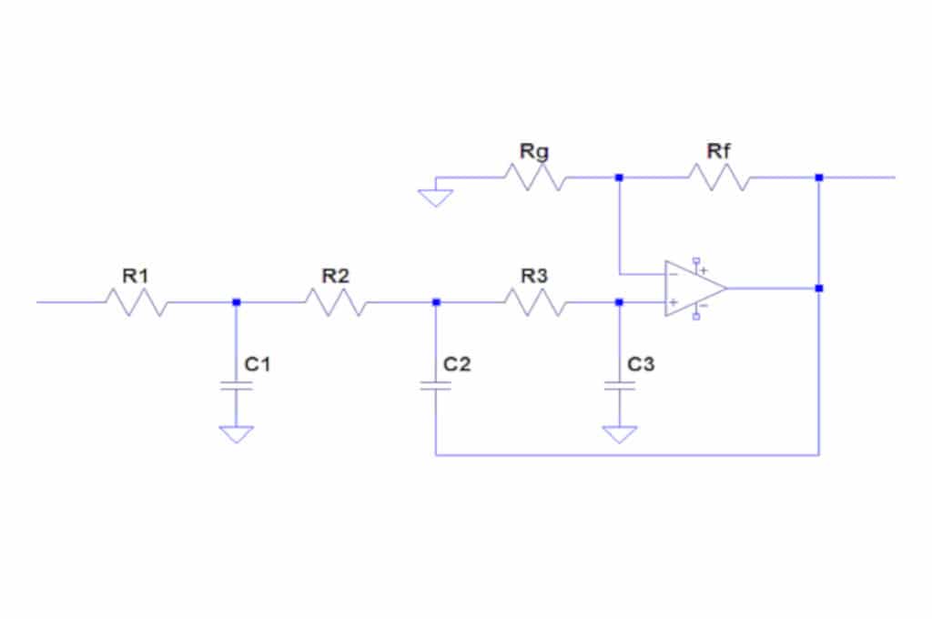
Figure 1 shows a third order low pass Sallen-Key filter implemented with a single op amp.
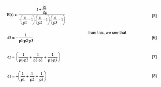
In analyzing this filter, I’ll take a slightly different path from the one pursued in the original article. The transfer function of this circuit is given by

A third order filter has three poles: p1, p2 and p3. One must be real, and without loss of generality, that will be p3. p1 and p2 can be real and identical, real and different, or complex. The real portions of all poles are negative, and if p1 and p2 are complex, their imaginary portions are negatives of one another.
Regardless of the nature of p1 and p2, we can always write H(s) as
One way to start to determine sets of component values which satisfy these equations is to solve [2] for R1 and substitute that expression into [3] and [4]. We can think of the result as two second order equations in R2:
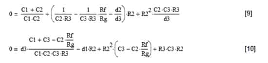
These are standard quadratic equations. Each yields two solutions for R2. The filter design requires that at least one solution to [9] be equal to at least one solution to [10]. But the six parameters other than R2 in these equations provide an overabundance of options for meeting that requirement. One approach that might tempt us would be to first normalize the equations so that the coefficient of the R22 terms in each was set to 1, and to then equate the coefficients of the R20 and R21 terms. This would result in two pairs of identical solutions. Unfortunately, this over-constrains the problem and limits the search for the best results. We don’t need two identical solution sets; we need only one solution that is common to both equations. That the normalization approach is undesirable is particularly frustrating in that equating coefficients simplifies the problem significantly by leading to algebraically tractable results – which are sadly non-optimal. A different approach for getting the best solution must be taken to properly constrain the problem so that it is manageable.
The selected successful strategy begins by limiting the component values under consideration to commercially available ones. IEC 63 (which evolved into IEC 60063) defines these values using something called an E-series. The E-x series specifies component value mantissas of 10i/x, where i is an integer from 1 to x, and x can be 3, 6, 12, 24, 48, 96 or 192. These mantissas are rounded to three digits for x ≥ 48 and two digits otherwise. (Because the values in the two-digit series were established before the IEC standard, not all of them follow this mathematical rule exactly.) Multiplying these mantissas by powers of ten yields available component values. Our strategy continues by setting the minimum and maximum values for to be considered for capacitors and resistors. Range limitations have practical value beyond reducing the number of component combinations. Few of us would want to design filters with 1 pF capacitors or 100 Megaohm resistors!
With these component value limitations in place, a computer program can iterate through all combinations to evaluate the two solutions each of equations [9] and [10]. The four sets of differences between an equation [9] and an equation [10] solution can be inspected for changes of sign between successive iterations. Such a sign change indicates that a solution from [9] and one from [10] are nearly equal. The component values from the iteration yielding the smaller difference in the R2 values is selected as a solution for consideration.
This approach can yield multiple solutions. How can we select the best among them? The answer is to evaluate the sensitivity of the filter’s amplitude response to the variations in the values of components (component tolerances) from their precise E-series specifications. The obvious choice for the evaluation point is the resonance frequency, at least when the poles p1 and p2 are complex, since this is the frequency of greatest response variation in that case. Regardless, any evaluation frequency can be chosen.
Sensitivity
The sensitivity of the amplitude response of a filter at frequency ω to variations in the value of component y is

Calculating the derivatives of this function for this filter is arduous. An acceptable alternative is to exploit the definition of a derivative and calculate differences instead, perturbing y by a very small fraction ε of its value, that is, multiplying it by delta = 1 + ε:

We can arrive at a measure of the sensitivity of the response to variations of all components by calculating the square root of the sum of the squares of the sensitivities to each of the individual component. But we must take into account the relative tolerances of each component if we are to select the solution with the least overall sensitivity. One way to do this is to multiply each individual sensitivity by the percent rating of the tolerance of its associated component. And so, we have the total sensitivity S for all i components yi:

With this figure of merit available, the solution with the best (least) sensitivity to component variations can be selected. For reference, the program also selects the solution with greatest sensitivity. LTSpice can do Monte Carlo runs on the designs for comparison purposes.
The program
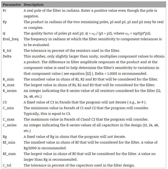
This program implements the algorithm described. It accepts the editable input text file 3rdOrderFilter.txt and asks the user to specify a name for the output file to which the contents of 3rdOrderFilter.txt are prepended. The required format and contents of the input file are self-documented. The following table supplies a summary of the input data that is required:
Since the program’s run time can extend into minutes, its progress in percent is continuously updated on the console. The program’s text file output includes the input file. To that it adds additional information, which is also displayed on the computer console. The output includes the total number of solutions found. It provides detailed information associated with the least and most sensitive solutions. Calculated values of R1 and R2 are displayed and used with the other component values (also provided) to calculate filter sensitivity. The nearest specified E-series component values of R1 and R2 are also presented along with the total filter sensitivity calculated using those component values. The E-series component values are then used to determine the percent errors in the coefficients of the powers of “s” terms in the denominator of H(s).
The program was run with the follow values in the input file:
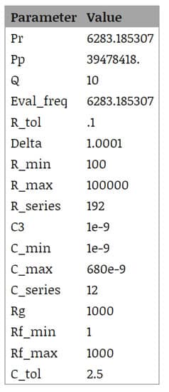
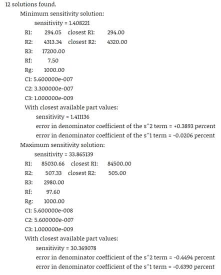
The program with the left table input file returned the following information:
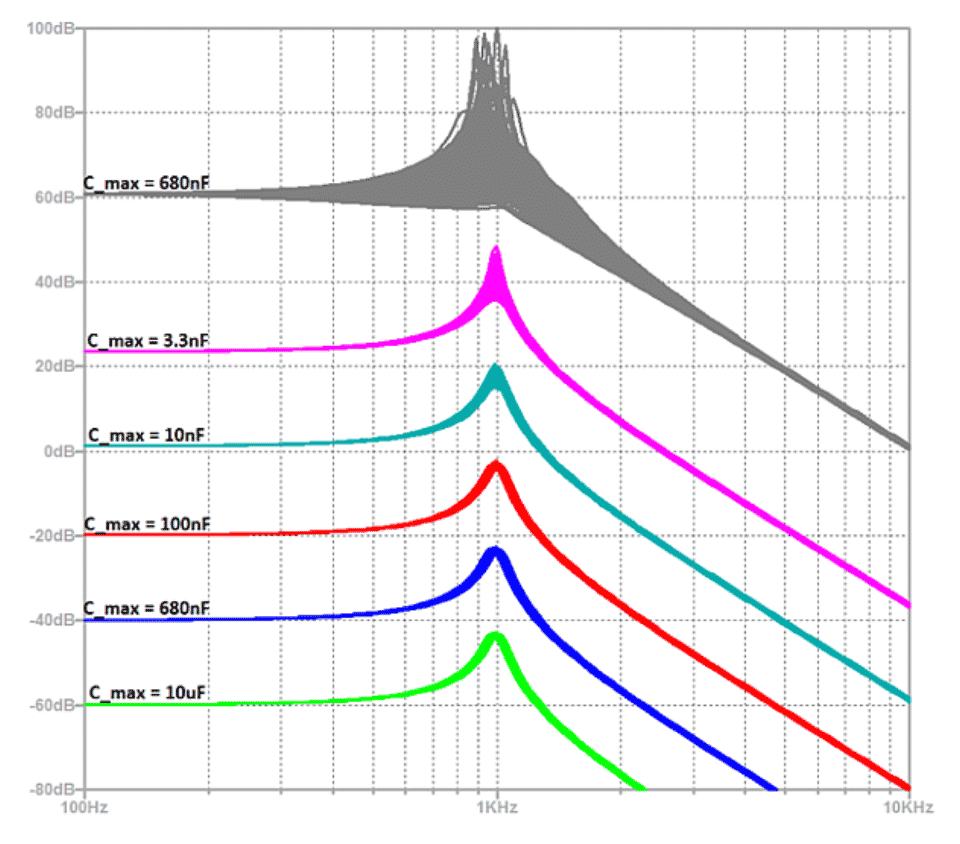
Several other versions of the program were run with larger and smaller values of C_max. An LTSpice 200-run Monte Carlo simulation of these designs yielded the following curves offset by multiples of 20dB so that they could be easily distinguished from one another. The curves are annotated with their C_max values. All are minimum sensitivity curves returned by the program except for the top one, which has the greatest variations:
Practical considerations for filter designs and running the program
Inspection of the curves on the graph reveals that low filter sensitivity benefits from the availability of a wide range of capacitor values (recall that C3 = C_min = 1nF.) However, there is also clearly a point of diminishing returns. And of course, 10uF 2.5% tolerance capacitors are not commercially available. Even if they were, they would be physically large and quite expensive. For this Q = 10 design, a maximum value 10nF 2% tolerance capacitor for $.05 in quantity is not an unreasonable choice.
Something else that becomes apparent when you examine equations [1] through [4]. Regarding Rf and Rg, their individual values don’t matter – only their ratio does. And when the range of available capacitors is large, very small Rf/Rg ratios lead to the lowest overall sensitivities. For that reason, Rf_min is recommended to be set to Rg/1000, even though that will extend the run time of the program. It has been my experience that there is little use to setting Rf_max to be larger than Rg for a DC gain greater than 2, and that higher sensitivities correlate with higher Rf/Rg ratios. But I cannot prove this.
In determining how to set input file parameters, the most important considerations are probably related to cost and availability. Chief among these is the budget for the more expensive components, the capacitors. They have the largest tolerances and the highest costs, and probably the largest PCB footprints. Setting the limits on these will probably have the biggest effect on filter sensitivities.
As for resistors, the 1% E96 resistors are most likely the best compromise between cost and accuracy of the coefficients of the powers of s in the denominator. They are available at lower costs and offer superior resolutions in values to those of the capacitors.
Probably least important is setting the input file parameters with consideration to the program run times. Choosing lower valued E-series and smaller ratios of maximum to minimum component value ratios will lead to shorter run times, but we’re talking minutes here, not hours. It’s probably best to choose these parameters based on cost, size, availability, and the extreme values that the design will tolerate, start the program running and go out for a cup of coffee, tea, or your favorite alternative poison. Life is too short to watch the “percent complete” counter advance on the screen.
In conclusion. a program has been written and offered to determine practical component values to implement a single op amp Sallen Key third order low pass filter. The user specifies the filter poles and acceptable ranges of component values. The program iterates through commercially available values to find the ones that yield a filter amplitude response that is the least sensitive overall to variations in component values due to tolerances. It also calculates the relative sensitivities and the accuracies of the coefficients in the denominator of the filter transfer function.
I welcome feedback on experiences with using this program. If there is sufficient interest, programs could be written for other topologies such as MFB or response types such as bandpass or lowpass.
Christopher Paul has worked in various engineering positions in the communications industry for over 40 years.