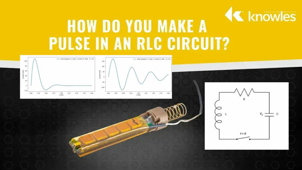
This article based on Knowles Precision Devices blog explains how an RLC circuit responds to a switching pulse.
One of the fundamental roles of capacitors is charging and discharging energy predictably. Many electronics applications leverage capacitors to store energy and release it in a controlled pulse of current or voltage. Here, we’ll revisit how pulses are produced in a basic RLC circuit featuring a capacitor (C), inductor (L) and resistor (R).
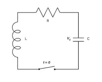
Series RLC Circuit
As mentioned above, a series RLC circuit, show in Figure 1, is made up of the three most common passive components in electronics engineering. When the capacitor is charged to an initial voltage (V0) and switched to discharge via the resistor and inductor (I0=0), three types of responses can occur depending on the component values involved.
When assessing current in an RLC circuit, damping dictates which equation you should use to determine how current varies over time. Is the system overdamped, critically damped or underdamped? The damping ratio, ζ, places a system into one of these categories.
Two RLC circuit parameters can be used to understand a system’s damping ratio: neper frequency and resonant angular frequency.
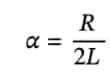
Neper Frequency
The neper frequency refers to an exponential transience rate. In other words, how quickly is energy lost from the system?
Find the neper frequency α using:
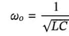
Resonant Angular Frequency
The resonant angular frequency ω0 indicates what frequency a system will oscillate at:
In combination, these parameters can be used to calculate the damping factor and identify which mathematical model would best represent the system’s behavior.
Damping Factor
Refocusing on the damping factor, the value for ζ places the system into one of three categories. There are three cases to consider:
Case 1: Overdamped: ζ > 1
Case 2: Critically Damped: ζ = 1
Case 3: Under Damped: ζ < 1
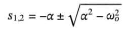
where:

Capacitor Discharge Current Theory derives solutions for current over time for each damping case. Here, we’ll leverage those results for the sake of example.
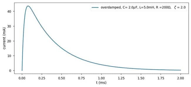
Case 1: Overdamped Current Response
When ζ > 1, apply the following equation:
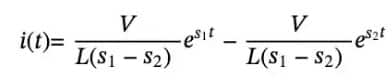
where:
To observe an overdamped response, shown in Figure 2, charge the capacitor to 10V and set C to 2.0μF, L to 5.0mH and R to 200Ω.
Case 2: Critically Damped Current Response Case 3: Underdamped Current Response
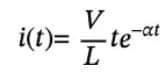
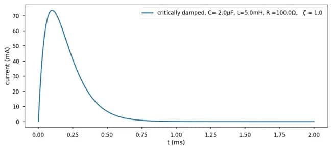
When ζ = 1, apply the following equation:
To observe a critically damped response, shown in Figure 3, keep C and L the same and set R to 100Ω. As shown, critically damped cases typically have higher peak amplitudes than overdamped cases.
Case 3: Underdamped Current Response
When ζ < 1, apply the following equation:
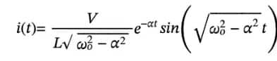
To observe an underdamped response, shown in Figure 4, keep C and L the same and set R to 50Ω. With all over variables remaining constant over time, resistance drives damping. As resistance decreases, the damping ratio decreases and peaks get larger. In this case, oscillation and decay, a pair known as ringing, become more pronounced too. The damping ratio determines the rate at which decay occurs.
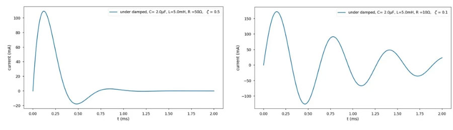
Peak current varies among damping cases, which is best observed on a single plot, Figure 5.
The Impact of Capacitance on Circuit Response
Changing resistance (Figure 3) has the most significant impact on damping ratio; however, changes in capacitance and inductance can also change the shape of the system response.
Consider the earlier equation:
where,
By rewriting ζ in terms of α and ω, you have:
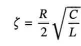
The damping ratio was 2.0 when values were set to C = 2.0µF, L = 5.0mH and R = 200Ω. By changing C to 1.0µF, the damping ratio is approximately 1.41. Since this is still considered an overdamped condition, you can use the equation for an overdamped case to compare 2.0µF and 1.0µF of capacitance, Figure 6.
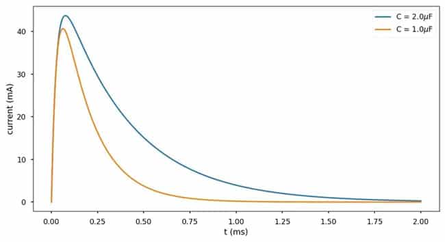
The area under 1.0µF capacitance case is smaller, which is reasonable to expect from a smaller capacitor that stores less charge.
Here, we’ve explored:
- The three relevant equations for current waveform in an RLC circuit
- The cases in which those equations are valid (depending on the damping ratio range)
- How adjusting the capacitance value in the RLC circuit changes the shape of the waveform