This blog article from Knowles Precision Devices explains filter poles and zeros. In this article we go in-depth on the background information of how poles and zeros impact a transfer function to show how this information can be used to improve filter’s performance.
n previous article Filter Q Factor Explained we discussed the different ways you can look at Q factor, one of which is to consider the Pole Q factor (often used with more complex systems).
We also explained in that post that filters have a transfer function H(s) which tells us what an output signal will look like for a given input signal. Note that filter transfer functions are expressed in terms of the complex variable ‘s’.
Poles and zeros are properties of the transfer function, and in general, solutions that make the function tend to zero are called, well, zeros, and the roots that make the function tend towards its maximum function are called poles.
Let’s look at how this works using a simple RC first order lowpass filter, like the one we looked at Basic Filter Circuits Explained (Figure 1).

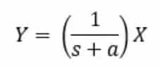
The transfer function for this filter written in terms of the complex frequency s, is as follows:
Thus, when s (frequency) = 0, the transfer function is 1 and we say the filter has a DC gain of 1. At s = -1/RC the transfer function will tend to infinity, so we say we have a single ‘pole’ at frequency s = -1/RC.
Now, knowing there is a ‘pole’ at s = -1/RC really does not help us understand how the filter performs versus frequency ω, not yet anyway. To determine this, we are going to look at a more general transfer function for a first order filter:
Then to understand the frequency response we replace s with jω, where j is the imaginary number “i“:
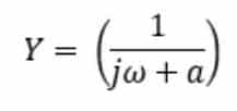
When jω = -a the transfer function tends to infinity, and we say we have a pole.
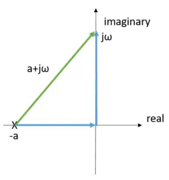
Next, if we plot the pole at -a in the complex plane of the ‘pole zero’ plot and mark it with an X, you get the graph shown in Figure 2. To see how the transfer function behaves at different values for frequency we can move the frequency value up and down the imaginary (vertical) axis for different values of jω see Figure 2.
Our transfer function will perform in the following manner – as the distance from the pole at to the frequency we are interested in grows, the signal will decrease since we are dividing by the size of that green vector (a+jω). Some additional general notes about this transfer function:
- at jω = 0 – We are as close to the pole as we can get if we stay on the imaginary axis and our transfer function Y will be at a maximum.
- at jω = ∞ – We are as far away from the pole as we can get, and our transfer function Y will be at a minimum.
- at jω = a – Our amplitude will be down by a ratio of √2 compared to its maximum, so in dB this is -3dB and we can say that is our cutoff frequency.
Therefore, in this simple case, our pole at -a gave us a cutoff frequency at a.
Similarly, our RC filter above with a pole at -1/RC gives us a cutoff frequency of ω = 1/RC.
This makes sense and we probably already know this is the cutoff frequency of an RC filter, but getting there via a roundabout route through a pole zero plot can help us understand how poles impact filter behavior.
Using Pole and Zero Information to Enhance Your Filter Designs
Through this single pole example, we can make the following general observation about poles:
- The closer your frequency of interest puts you on the complex plane relative to a pole, the filter’s transfer function will increase
- The further you are away from a pole and the filter’s transfer function will decrease
- Zeros have the opposite effect – the closer your frequency puts you to a pole, the filter transfer function will decrease and vice-versa.
As an RF designer, if you have an in-depth understanding of how poles and zeros work, you can take advantage of this information in your filter designs and improve your filter’s response. For example, you can place zeros near frequencies you want to reject and poles near frequencies you want to pass.