


Magnetic components such as inductors and transformers are central to every switched‑mode power supply, yet their design is notoriously difficult to get right without extensive prototyping.
This article based on Frenetic webinar explains, in practical engineering terms, how a modern simulator can model magnetics and inductors from first principles, using Frenetic’s approach as a concrete example while keeping the concepts general enough for design engineers and component specialists.
Why Magnetic Modeling Matters
Designers rely on models to predict inductance, losses and temperature before committing to hardware, PCB layouts and mechanical integration. Good models help reduce the number of prototype spins, avoid overheating, and prevent last‑minute surprises around saturation or unexpected leakage. Understanding the assumptions behind these models also shows when analytical formulas are sufficient and when more advanced numerical methods such as finite‑element analysis (FEM) are justified.
Analytical Models vs FEM in Magnetics
In industry, FEM simulations have a reputation for being “the most accurate” way to model inductors and transformers, but the reality is more nuanced. FEM excels at solving electromagnetic fields for arbitrary geometries and is particularly strong for winding losses in complex arrangements, yet it struggles with nonlinear core losses and can be slow for everyday design work. Analytical and semi‑empirical models, when used within their validity range, can be both accurate and far more efficient, making them better suited for iterative design and optimization.
Modeling Approaches at a Glance
| Aspect | Analytical / Semi‑empirical model | FEM‑based model |
|---|---|---|
| Geometry | Standard cores, regular windings | Arbitrary, complex geometries |
| Losses handled well | Core loss (IGS), many winding types | Detailed winding loss, local field effects |
| Computation time | Fast, suitable for iteration | Slower, heavier setup |
| Typical use | Early design, parametric sweeps | Planar magnetics, edge cases, validation |
| Main limitation | Assumptions on field distribution | Nonlinear loss modeling, simulation effort |
A practical strategy is to use analytical methods for the bulk of designs and reserve FEM for difficult geometries, especially in planar magnetics.
Building a Magnetic Circuit Model
Reluctance as the Magnetic “Resistance”
The starting point for many magnetic models is the reluctance network, which is the magnetic analogue of an electrical resistance network. The magnetomotive force is given by and drives a magnetic flux through a network of reluctances representing the core, air gaps and leakage paths. Once the network is set up, the simulator can compute inductance as a function of current, flux density distribution in different core sections, and stray fields near the air gap.
Air Gap and Fringing
Air gaps are often the most critical and tricky part of the magnetic circuit, because the magnetic field “fringes” into the surrounding space instead of staying confined to the core cross‑section. Ignoring fringing leads to large errors in both inductance and saturation‑current predictions. A practical approach is to decompose the air‑gap region into analytical “building blocks” whose reluctances are known and assemble them like Lego bricks to approximate the real geometry, including fringing.
Core and Winding Losses in Practice
Core Loss with Improved Steinmetz Equations
Core losses depend on flux density, frequency, waveform shape and material properties. Many modern tools use improved generalized Steinmetz (IGS‑type) equations, which better handle non‑sinusoidal waveforms typical of switched‑mode power supplies. In practice, the simulator takes the flux‑density waveform, splits it into segments, applies the material‑specific IGS parameters to each segment, and integrates over one period to obtain total core loss.
Winding Losses, Skin and Proximity Effects
Copper loss is not just I2R when switching at tens or hundreds of kilohertz. Skin and proximity effects increase effective AC resistance and can dominate total loss, especially in tightly packed transformers and inductors. Analytical formulas exist for standard conductor types (solid wire, litz, some foil geometries) as long as the external magnetic field around each conductor is known.
One efficient method computes this external field by:
- Replacing the air gap with an equivalent current source that reproduces the same field.
- Using the method of images to mirror conductors across core boundaries, building an infinite periodic arrangement.
The field at each conductor follows from superposition of all real and image conductors, after which known AC‑loss formulas provide winding losses.
When Planar Magnetics Need FEM
Planar magnetics, particularly PCB‑based transformers and inductors with thin rectangular traces, are a difficult case for pure analytical models. Strong field components orthogonal to the traces can drive high eddy currents, and deriving general closed‑form expressions for arbitrary PCB patterns is challenging. For these components, it is practical to move to FEM‑based models for losses and capacitances, while still using analytical or semi‑analytical methods for conventional wound components.
Compact Thermal Modeling and Iteration
After obtaining core and copper losses, the simulator needs to estimate temperature rise, which feeds back into material properties and loss coefficients. A simplified thermal equivalent circuit with thermal resistances between winding, core and ambient is often sufficient. Losses are applied as heat sources, temperatures are computed, and the process is iterated because losses themselves depend on temperature (for example through copper resistivity and core‑loss coefficients).
Electrical to Thermal Flow
| Step | What happens in the model |
|---|---|
| 1. Electrical excitation | Voltage, current, frequency defined |
| 2. Magnetic solution | Flux, inductance, fields, gap/fringing |
| 3. Loss calculation | Core loss, copper loss (AC and DC components) |
| 4. Thermal solution | Hotspot temperatures from RC thermal network |
| 5. Iteration | Update temperature‑dependent parameters and repeat |
For early design screening and optimization, this compact thermal loop is usually accurate enough to highlight thermal bottlenecks and guide geometry changes.
Design‑In Notes for Engineers
When using or reviewing results from a tool that follows this approach, consider:
- Check the core material and loss model; results rely on correct Steinmetz/IGS parameters.
- Look at how air gaps are modeled; poor fringing treatment can make inductance and saturation current too optimistic.
- For high‑frequency designs, pay attention to conductor type and how AC resistance is modeled (wire, litz, foil, PCB).
- Verify thermal boundary conditions such as cooling method, orientation and ambient temperature.
- For planar magnetics or very compact designs, confirm that FEM or equivalent advanced field modeling is used for loss and capacitance.
Understanding these blocks helps design engineers interpret simulation reports and gives component engineers a better basis for discussing custom magnetics proposals.
Typical Applications
The modeling concepts described here are directly relevant to:
- Flyback, forward, LLC and other isolated DC‑DC converters.
- PFC chokes and boost inductors.
- Output chokes and filter inductors in point‑of‑load regulators.
- Planar transformers in high‑density, low‑profile supplies.
- Magnetics in automotive and industrial drives with tight thermal margins.
Source
This article is based on a technical webinar presentation by Jonas Mühlethaler, CTO of Frenetic and Professor of Electrical Engineering at Lucerne University of Applied Sciences and Arts, describing a practical framework for modeling magnetic components from reluctance and loss calculations through to thermal predictions, and explaining why planar magnetics often require FEM due to their geometric complexity.