


Planar magnetics are an attractive option for high‑density power converters thanks to their low profile, excellent repeatability and large surface area for heat transfer. However, their thermal behavior is far from trivial, and inaccurate temperature modeling can easily lead to severe over‑ or under‑design.
This article based on edited blog by Dr.Molina, CEO of Frenetic, summarizes key insights from recent research on planar magnetics thermal modeling and translates them into practical design‑in guidance for magnetics and power engineers.
Key features and benefits of planar magnetics in thermal terms
Planar transformers and inductors differ from traditional wound components not only mechanically, but also thermally. Their geometry has a direct impact on how losses translate into temperature rise.
Thermal‑related characteristics of planar magnetics
- Large, flat surfaces in the core and copper structure enable efficient heat spreading and make them inherently suitable for heatsink or cold‑plate coupling.
- Short thermal paths from copper and core to ambient or to a cooling plate help reduce hot spots compared to bulky wire‑wound parts.
- Strong thermal coupling between layers leads to more uniform internal temperatures, which simplifies derating and reliability calculations when properly modeled.
- At the same time, the compact stackup can concentrate losses and cause steep temperature gradients if cooling and layout are not carefully engineered.
Why thermal modeling accuracy matters
- Copper and core losses are highly temperature‑dependent; underestimating temperature rise can lead to runaway effects and premature insulation or core material degradation.
- Overly conservative models can force oversizing of core and copper, undermining the main benefit of planar magnetics: achieving very high power density in a limited volume.
- Realistic thermal prediction is essential to meet safety standards, insulation class limits and lifetime targets in automotive, industrial and telecom power systems.
Typical applications where temperature modeling is critical
Planar magnetics are commonly used in converters where high power density, low profile and repeatability are more important than one‑off cost of the magnetic design itself. In these environments, thermal margins tend to be tight and ambient conditions harsh.
Representative application areas
- High‑power isolated DC‑DC converters in telecom and datacenter power shelves (e.g., 1–5 kW bricks, intermediate bus converters).
- On‑board chargers and DC‑DC converters in electric vehicles, where ambient and coolant temperatures vary widely and thermal cycling is severe.
- Industrial drives, servo drives and inverters, with continuous high load, elevated cabinet temperatures and limited airflow.
- Server and edge‑computing power supplies with aggressive height limits and stringent efficiency requirements.
- Wide‑bandgap‑based converters (SiC, GaN) running at higher switching frequencies, which push magnetic losses while enabling very compact layouts.
Typical circuit positions
- High‑frequency isolation transformers in full‑bridge, dual active bridge or LLC stages.
- Boost or PFC inductors in front‑end power factor correction stages.
- High‑current output inductors in multiphase DC‑DC regulators.
- Integrated planar magnetics structures combining transformer and inductors in a single core and PCB stack.
In all of these positions, inaccurate thermal modeling can translate directly into unexpected core saturation at elevated temperature, degraded efficiency, or failure to meet component and system qualification tests.
Technical highlights: methods for modeling planar magnetics temperature
Recent work on planar magnetics thermal modeling emphasizes that there is no single “silver bullet” method. Instead, a hierarchy of approaches exists, each with its own complexity, accuracy and error sources.
Three main approaches to thermal modeling
- Thermal resistance network models
- Represent the magnetic structure as a network of thermal resistances linking loss sources (copper, core, PCB) to ambient or coolant.
- Analytical or semi‑analytical; relatively accessible and fast to evaluate once the network and parameters are defined.
- Particularly useful in early design and optimization loops where many variants must be compared.
- However, they rely heavily on empirical or simplified parameters for convection and conduction, which can lead to significant error if not calibrated.
- Finite Element Method (FEM) thermal simulation
- Solves the heat conduction equation inside solid regions (core, copper, PCB, encapsulant) with boundary conditions based on heat transfer coefficients.
- Captures non‑uniform loss distribution, complex geometry and detailed material properties.
- Offers significantly improved accuracy over lumped thermal networks when properly set up and validated.
- Computationally more intensive and requires expertise in meshing, material modeling and boundary condition definition.
- Coupled fluid‑thermal simulations (CFD)
- Combine solid conduction models with detailed simulation of airflow or liquid flow around and through the magnetics assembly.
- Provide the most accurate representation of forced convection and local hot spots in complex system environments.
- Very powerful for final verification or for high‑risk designs, but also the most complex and time‑consuming approach in terms of modeling effort and runtime.
Three main strategies to remove heat
The cooling concept used with planar magnetics has a major impact on the achievable power density and the realism of thermal models.
- Natural convection
- Relies purely on buoyancy‑driven air movement around the component.
- For planar magnetics, natural convection alone usually cannot take advantage of the large surface area, especially when components are enclosed in tight housings.
- Typically not recommended as the only cooling method for high‑power planar transformers and inductors.
- Forced air cooling (fan‑based)
- Improves convection coefficient compared to natural convection, but the improvement for flat, low‑profile planar structures may be limited if airflow is constrained or poorly directed.
- May be reasonable for moderate power densities, but often insufficient for the most aggressive planar designs.
- Heatsink or liquid cooling
- Connecting the planar magnetic to a heatsink or cold plate (including liquid‑cooled plates) leverages its large contact area to remove heat efficiently.
- Offers a dramatic increase in effective heat transfer coefficient compared to air‑based cooling, enabling much higher power densities.
- Particularly attractive when the system already includes a liquid cooling loop for semiconductors or other high‑power components.
The evolution of convection coefficients from natural convection to forced air and water is dramatic:
| Material | Natural convection | Forced convection |
|---|---|---|
| Air | 5–30 | 100–300 |
| Water | 100–1000 | 300–12000 |
Scientific error and uncertainty in thermal modeling
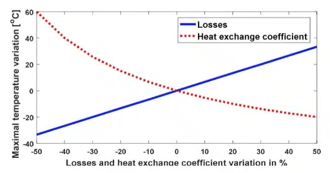
A key insight from recent research is that the error introduced by uncertainties in thermal parameters is far from negligible.
- Typical convective heat transfer coefficients, material thermal conductivities and contact resistances come with unavoidable tolerances.
- When these uncertainties are propagated through the model, the resulting temperature prediction can vary over a wide range, with deviations on the order of several tens of degrees Celsius.
- For planar magnetics, reported studies show that combined tolerances can produce temperature estimation errors roughly between −20 °C and +60 °C depending on the scenario and modeling approach.
- Such wide error bands underline the need to treat thermal models as decision‑support tools rather than absolute truth, and to validate them with measurements whenever possible.
| Class | Min −50% | Typical | Max +50% |
|---|---|---|---|
| Ferrite thermal conductivity [W·m⁻¹·K⁻¹] | 1.75 | 3.5 | 5.25 |
| Insulator thermal conductivity [W·m⁻¹·K⁻¹] | 0.075 | 0.15 | 0.225 |
| Copper thermal conductivity [W·m⁻¹·K⁻¹] | 200 | 400 | 600 |
| Total losses [W] | 3 | 6 | 9 |
| Heat exchange coefficient [W·m⁻²·K⁻¹] | 5 | 10 | 15 |
Availability of tools and recommended design targets
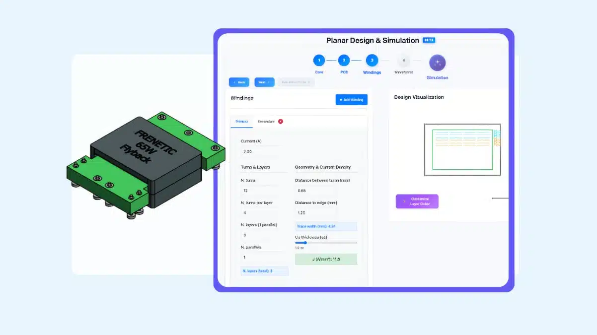
Modern magnetics design workflows increasingly couple loss calculation with thermal modeling, sometimes embedding FEM engines inside user‑friendly tools.
- Specialized design platforms for planar magnetics can automate copper and core loss calculation for given waveforms, geometries and materials, then feed these losses into internal FEM models.
- This combination provides a more realistic view of temperature rise than simple spreadsheet‑based thermal resistance models, especially in complex stackups or when cooling is non‑uniform.
- Using such a loss‑plus‑thermal co‑simulation workflow is particularly valuable in early design phases, where exploring several core and layer arrangements is necessary.
A practical typical target design for planar magnetics design is to aim for a power density of about 50 kW per liter of core volume as a reasonable goal for high‑performance planar transformers in demanding applications, provided that cooling and thermal margins are handled correctly and that the exact value is verified according to the manufacturer datasheet and design constraints.
Make sure your losses are accurately calculated. Recommendation: using Frenetic Planar with FEM running underneath is a solid approach:
Design‑in notes for engineers
This section summarizes practical guidance from the research and field experience to help engineers integrate planar magnetics with robust thermal behavior.
1. Understand and respect the limitations of each modeling method
- Use thermal resistance networks during early concept evaluation, but be aware that they often overestimate temperature rise due to conservative parameters and simplifications.
- Reserve FEM for detailed design and verification of shortlisted candidates, especially when the geometry is complex or when small temperature margins must be justified.
- Consider fluid‑thermal simulations when the system environment (enclosure, airflow, cold plates) plays a dominant role and when failure to meet thermal limits has high consequences.
2. Prioritize efficient cooling concepts from the beginning
- Plan for heatsink or cold‑plate mounting early in the mechanical design to fully leverage planar magnetics’ flat surfaces.
- When a liquid cooling loop is already available for power semiconductors, consider coupling the planar transformer or inductor to the same cold plate instead of adding fans.
- Design the interface (thermal pads, clamping, aluminum cover) to minimize contact resistance and ensure uniform pressure across the surface.
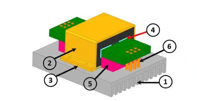
3. Use mechanical features to homogenize temperature
Adding an aluminum cap or cover over the planar core brings several benefits:
- It helps to homogenize temperature across the component by spreading heat between hot and cooler regions.
- It improves the thermal contact area towards the heatsink or cold plate, reducing local hot spots.
- It can also offer mechanical protection and EMI shielding if properly designed and grounded, which is relevant for planar structures with large copper areas.
4. Ensure accurate loss calculation before trusting any thermal result
Thermal modeling quality is directly linked to the quality of the loss input data.
- Use realistic waveforms and switching conditions for both copper and core loss calculations.
- For copper losses, include skin and proximity effects, which are especially pronounced in planar conductors and multilayer PCB structures.
- For core losses, rely on manufacturer‑provided Steinmetz or improved models within their specified frequency and flux density ranges, and validate that operating points remain inside recommended limits according to the manufacturer datasheet.
- Feeding these detailed loss distributions into FEM greatly improves the credibility of the resulting temperature maps.
5. Validate models with measurements and keep safety margins
Given the large potential error in thermal parameter assumptions:
- Instrument prototypes with thermocouples or infrared measurement to validate simulated temperature distributions under worst‑case operating conditions.
- Compare measured and predicted hot spot temperatures, and adjust model parameters (e.g. convection coefficients, contact resistances) to better match reality.
- Maintain adequate safety margins between the maximum observed or predicted temperatures and the limits defined by insulation class, core material and surrounding components.
6. Coordinate electrical, thermal and reliability targets
Planar magnetics thermal design does not stand alone; it is tightly linked to electrical performance and lifetime requirements.
- Higher permissible temperature may allow higher power density, but also accelerates insulation aging and may increase core loss.
- Conversely, overly conservative temperature limits might force larger core sizes and increase stray capacitances, impacting EMI performance.
- Aim for a balanced design where the chosen cooling strategy, modeling approach and power density target are consistent with system‑level efficiency, cost and reliability goals.
7. Practical selection hints for purchasing and component engineering
For purchasing teams and component engineers working with planar magnetics suppliers:
- Request thermal characterization data and example models from suppliers, including recommended convection coefficients or mounting guidelines.
- Clarify recommended maximum winding and core temperatures and how they were determined.
- Ask whether suppliers offer FEM‑based design support or co‑simulation services to validate critical designs.
- Ensure that the chosen core and PCB technology can meet the required power density objectives under the available cooling concept, according to manufacturer datasheet and test data.
Source
The information and design guidance in this article are based on a recent in‑depth tutorial on planar magnetics thermal modeling and on the underlying IEEE research paper on thermal modeling of planar magnetics, complemented by practical engineering interpretation for power electronics applications.