source: EDN article
Mark Stansberry -July 30, 2017
If you want to replicate the music of your favorite musicians, you will need to know the pedal effect devices they use and the circuitry within them. Furthermore, if you want to design new pedal effects that please your audience, you will need the right tools, the right design flows, the right components, some circuit know-how, and a little creativity.
The design of pedal effect circuits, i.e. circuits that modify the waveforms of musical instruments, is an art and science that has been practiced since the 1920s. Fundamental to the reproduction of era-specific and musician-specific music is the technology contained in these pedal effect gadgets. Different artists prefer different component technology: tubes, germanium transistors, silicon bipolar transistors, MOSFETs, diodes, JFETS, op amps or any mix thereof.
The passive components used in pedal effect circuits, like inductors, capacitors and resistors, complicate the process of analog sound reproduction. Of specific mystical interest to many professional musicians is the “magical inductor.” Thought to be enchanted music’s key, the magical inductor, once placed inside a circuit generates harmonics that separate it apart from all other inductors. The idea of a magical inductor keeps musicians wondering. Is music’s holy grail locked inside the pedal device of a long-ago musician? Is the magical inductor made of a special material? Is the magical inductor lost in time and do the music giants of our times have access to it? One thing most of them agree on is that the magical inductor is one of the analog Muses and not one of the digital Sirens.
Audio circuit simulation and emulation
Audio engineers and musicians use a variety of tools to help them create analog pedal effect circuits. Among those are Digital Audio Workstations (DAW) and analog circuit simulators such as LTspice. Using these two tools together, designers can electrically analyze and listen to different wave modification circuits without building the circuitry.
These two tools give the audio designer different design flow options. Instead of design, simulate, build, and test, the designer has the exploratory option of design, simulate and emulate. After the pedal effect circuit schematic is entered into the LTspice circuit simulator and after it is simulated for basic electrical performance characteristics, such as bias, gain, noise, harmonics and frequency response, it is run through an audio emulator (which could be an expensive DAW software package or a free multimedia player). For an audio emulation, a music file such as a WAV or MIDI file is fed into the LTspice circuit simulator. The audio output file from LTspice is then played with a DAW or multimedia player and listened to on a pair of high-quality headphones.
Although this is an efficient way to listen to the circuit performance without building the circuit, the audio emulation will not necessarily produce an exact replica of the analog circuit. You could very well lose analog subtleties and associated music intonations that the actual analog circuit produces.
When the designer uses his or her ear, and musical and circuit analysis experience, the designer can mentally interpolate how the audio emulation will actually sound when it comes out of an analog circuit. To a large extent, audio mental interpolation takes experience to do well. To gain this experience, once a pedal LTspice circuit’s harmonics are examined and listened to on a DAW or media player, the designer should build and listen to the actual hardware prototype with, for example, a guitar as its input. Developing audio mental interpolation skills also requires that the actual hardware prototype waveforms on the oscilloscope be compared with the DAW’s output and the sound you hear. In this way, the designer can determine what is lost in the LTspice/DAW audio emulation harmonic analysis (Fast Fourier Transform).
Pedal effect design
There are literally thousands of different pedal devices and variants on the market. Some of the most popular effects include distortion, fuzz, overdrive, the Wah, delay, flanger, boost, phaser and tremolo. There are also hundreds of different ways to create a pedal circuit. Musicians often favor pedal effect circuits created with specific types of components or with a specific circuit design; that’s because the subtleness of the sound will often depend on the specific circuit design and the types of components used.
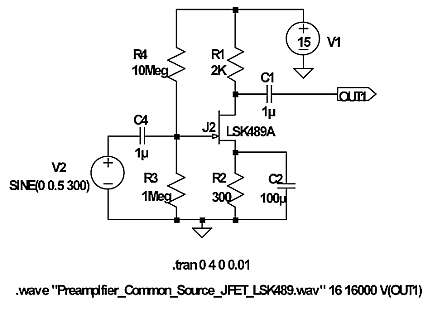
A distortion pedal effect circuit is relatively simple to build. A basic one-transistor amplifier can be used. However, unlike the design of an amplifier, where the goal is to produce an exact duplicate of the input waveform with little or no distortion, the design goal of the pedal distortion circuit is to add just the right amount of distortion. There are several ways to do this. The most common is to alter the bias point of the amplifier. In the JFET amplifier design below, the bias resistors, and the source and drain resistors can be varied to introduce different levels of distortion. Another common way is to overdrive the amplifier. One more way is to modulate the voltage supply.
In the circuit that follows, a common source amplifier configuration was used. It was designed to introduce as little distortion as possible. Specifically, a bias point and a low enough input voltage level was used to avoid clipping. The JFET was selected because it, of all discrete transistor devices, mimics the operation of the now-ancient vacuum tube.


To capture the audio with LTspice, as shown in Figure 1, a wave statement was used as a SPICE directive:
.wave “Preamplifier_Common_Source_JFET_LSK489” 16 16000 V(Out1)
The statement specifies the audio output wave file that the audio output is to be stored in, Preamplifier_Common_Source_JFET_LSK489.wav. The command also specifies 16-bit resolution sampling, 16,000 samples per second sampling rate and the node to be recorded, Out1 (the output node of the amplifier). LTspice allows for sampling rates up to 4 billion samples per second (1), way more than you will need for high quality audio and video recording!
With a 300 Hertz, 0.5Vpp input signal, the common source amplifier outputs a 300 Hz signal (4.5 Vpp) that is 180 degrees out of phase with the input (Figure 2). If you do not want the phase shift, you would have to include another common source amplifier (the LSK489 contains two JFETs per package) to introduce another 180-degree phase shift or use a common drain or gate configuration.

To introduce some overdrive distortion, the input signal is increased to 3 volts peak-to-peak. The resultant output waveform is given below. As can be seen, it is asymmetrically clipped at the top (2).

When the distorted and non-distorted waveforms are listened to and compared on Microsoft’s Media Player you can discern the difference. The clipping reduces the bass and increases the pitch (attributed to the higher level of the 2nd and 3rd harmonics).

The audio files, preamplfier_common_source_jfet_lsk489.wav and hard_clipping_jfet_lsk489_15volt.wav, are the audio from the output waveforms in Figures 2 and 3. They can be listened to on a DAW or if you’re on a budget, on your Windows Media Player, which comes preinstalled on almost all PCs.
With the LTspice schematic (Figure 1), it is easy to hear how component changes will affect the audio output. Simply change a component, rerun the simulation, and then listen to the new wav file. You can also easily hear how different sampling rates will affect the audio quality. For example, if you want studio recording quality, changing the sampling rate parameter of the wave. statement from 16000 to 192000 samples per second (sps) will do the job. But you don’t have to stop there. If you want to hear how your own music will sound, you can reconfigure the input source in the LTspice schematic so that it will input your own wav file recordings.
Emulation advantages and precautions
Audio simulation and emulation with LTspice and a simple digital audio system, such as Windows Multimedia Players, gives pedal designers a tremendous design advantage. Analog emulation eliminates the expense and time associated with hardware prototyping. Analog emulation also opens the door to automated design flows. SPICE scripts can be written that cycle through component values, analyze output and report on favorable harmonic outputs. Analog emulation also facilitates an intuitive design approach that can override the time-consuming process of analog circuit analysis.
Caution, however, must be exercised. Digital emulation of audio signals may lose subtle harmonics. However, this loss can be overcome if ultra-high digital sampling rates are used. LTspice offers ultra-high sampling rates (Gsps), but for the real world a 192 Ksps with a 24-bit resolution, studio quality, will do. Other considerations are the quality of the amplifiers in an audio workstation and the headphones used. The sound circuit in the audio workstation should be able to play 192 Ksps music.
Care must also be exercised in the circuit design. Analog circuit simulators often don’t report violations of basic circuit design rules that can cause a circuit to fail. For example, the gate-to-source voltage of a N-channel JFET should always be less than zero. Large positive excursions above 0 V result in forward biasing the gate-to-source diode junction. An excessive forward bias voltage will eventually result in an inoperable JFET. Most analog circuit simulators do not report a design error if you exceed the maximum drain-to-source voltage.
References
- Processing Audio with Octave and LTspice, Author; Dr. Tony Richardson, Affiliation: University of Evansville.
- A Musical Distortion Primer, Author: R.G. Keens, Publisher: Geo-Fex Cybernetic Music, Publication Date: 1993.
- The LSK489 Data Sheet: Low Noise Low Capacitance Monolithic Dual N-Channel JFET Amplifier, Publisher: Linear Integrated Systems.
- Using WAVE files as input/output in LTspice
- LTspice Tutorial -how to use this program.
- Why are JFET based petals better than op amp based petals, Publication Date: April, 2013, Publisher: Tdpri.com
- Field Effect Transistors in Theory and Practice, Application Note AN211, Publisher: Motorola, Publication Date: 1993
- FETs versus Tubes: Exploding the Myths, Publisher: Diystompboxes.com, Publication Date: October 2010
Mark Stansberry participates in the technology and education industry as a writer, publisher, engineer, educator, and technical research and market analyst.