by Kenneth Wyatt. EMC engineers are often called on to design low-pass filters for client projects, which is usually required to meet radiated susceptibility tests. While the most common radiated-immunity standard (IEC/EN 61000-4-3) requires testing from 80 MHz to 1000 MHz, this case study required immunity from a nearby 50 W, 500 kHz source.
In this case, the prototype product included a simple “PI” filter, comprising a parallel 330 pF capacitor, a series ferrite bead, and a parallel 100 pF capacitor. The load was 4.02 kΩ.
I thought this would be a good time to use Linear Technology’s free LT SPICE software to perform some quick simulations. LT SPICE is a PC-based analysis software with a convenient schematic entry front-end. It’s also very easy to add voltage and current “probes” throughput your circuit to monitor the performance.
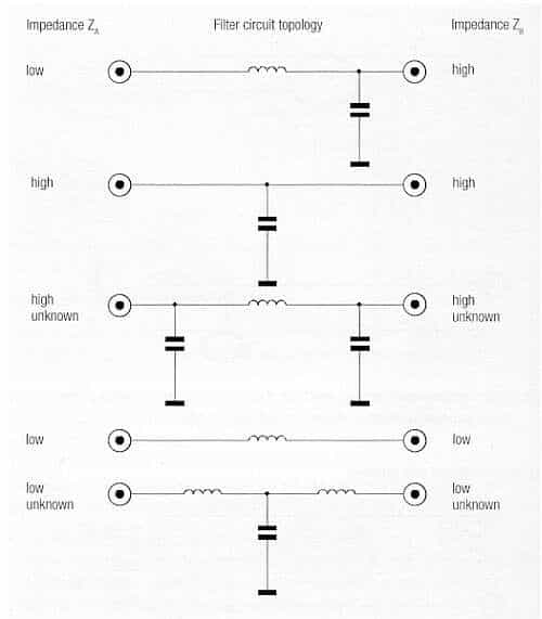
But first, which of the several filter topologies would be most appropriate? Würth Electronik has a very nice filter design section in its book, Trilogy of Magnetics. It turns out the right filter topology depends on the input and out impedances of the system. I’ve reproduced a handy chart (Figure 1) from page 184 of the book that you should copy and tuck into your lab notebook.
For the series filter impedance (the ferrite bead, in this case) to work, it must “see” a low impedance at each end. For example, placing a 200 Ω ferrite bead into a system with 1000 Ω and 4 kΩ input-and-output impedances wouldn’t offer sufficient series impedance to affect interfering signals. On the other hand, that same 200 Ω ferrite would work fine if the input and output impedances were near 1 Ω. That’s the purpose of the parallel capacitors.
In this case, the input impedance to the filter could vary, depending on the sensor impedance, and we knew the output impedance was 4.02 kΩ. The designer had already used a PI filter topology, which should perform well for any impedance from low to high, per the chart.

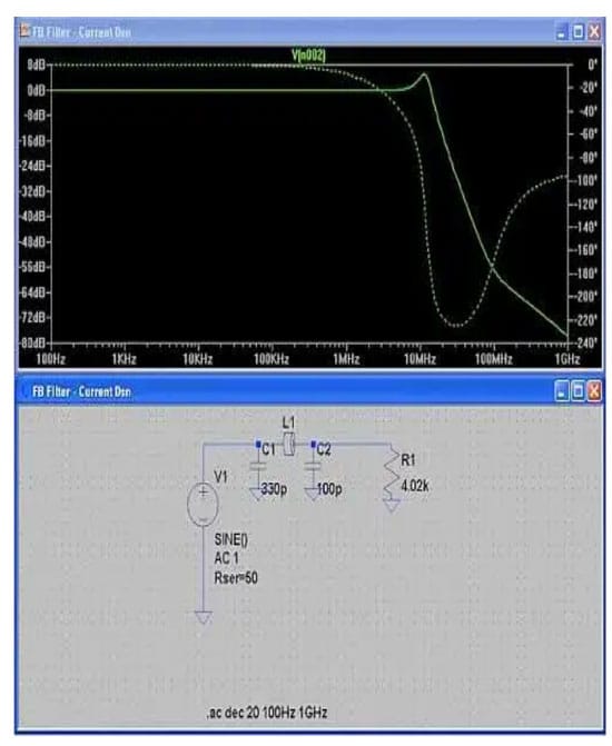
Here’s the original input filter circuit (Figure 2). For the purposes of this simulation, I ignored the Transzorb® D13. The input is on the left and output on the right.
By inspection, I could tell the current values of capacitors were way too small to provide a low impedance to ground for a frequency of 500 kHz, so the first thing I tried was to increase them to 0.47 µF, each. But first, let’s simulate the current circuit to see where the impedance starts to roll off.
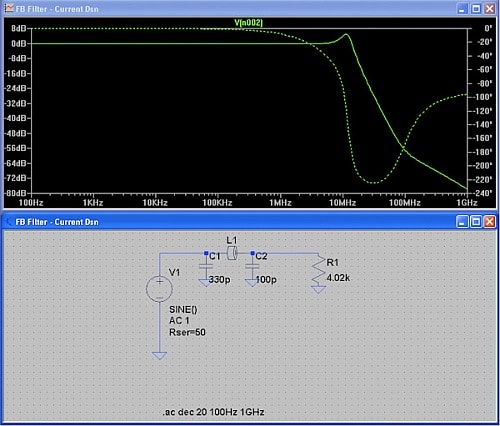
Here’s the LT SPICE simulation (Figure 3). I used an input impedance of 50 Ω, but with the proper valued capacitor, it really doesn’t matter much. Note that the 3 dB rolloff (solid line) occurs about 16 MHz; way too high to help at 500 kHz.
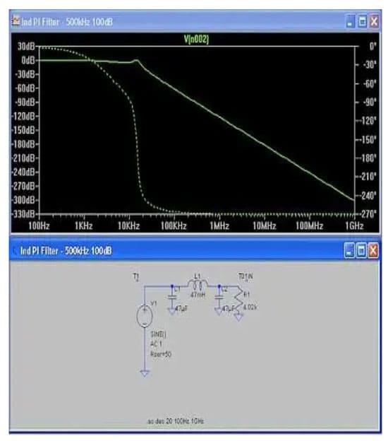
Here’s the final LT SPICE simulation with 0.47 µF capacitors and the ferrite replaced with a 0.47 mH inductor (Figure 4). Note the improved filter starts rolling off at 20 kHz — well below the critical 500 kHz interfering signal and provides about 90 dB of attenuation at 500 kHz. The client was able to use the same real estate on the PC board to mount the new components. While there were other circuit changes and better shielding required, due to the proximity of the source, the filter reduced the high level of interference.