This article based on Frenetic newsletter written by Jonathan Church, Frenetic product director, is exploring selection of core and transformer optimal operation conditions for phase-shifted full bridge converter. Updated 12th July 2023.
Phase-Shifted Full-Bridge (PSFB) configuration is a popular converter topology for its wide power handling range, isolation, control simplicity and its ability to take advantage of Zero Voltage Switching (ZVS).
To that end you’ll find it in many modern applications.
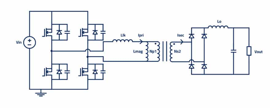
See Figure 1. for typical PSFB circuit topology.
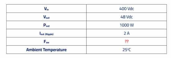
In this case study lets consider arbitrary and simple specification shown in Table 1, the less detail the better at this point.
Optimal Frequency for Power Converters
Finding the right balance between size and efficiency to achieve the greatest power density may be challenging. Selection of optimum operating frequencies may be a key design element here, but it requires a well-rounded understanding of your system.
Increasing the operating frequency will reduce converter size, but eventually the gains will be eroded by the need for additional heatsinking or other forms of more advanced and costly cooling. Alas, another plate to spin. Let’s take a holistic look at the effect that the changing of frequency has on our power system components below.
Intuitively, your switching losses and gate-drive losses are going to proportionally increase. Many great innovations are reducing the gradient to which these losses increase but despite this and despite any type of soft-switching resonant converter you may be using, this is still going to happen so keep an eye on them.
The reactive components in the system will reduce in size as you increase the frequency, notably your input and output filtering. This is a quick win for your power density providing you have well in hand (sorry Luke) the knowledge required to design an effective filter, plus you understand the control and stability aspects of your design.
Now let’s talk about the “bottleneck”, or perhaps a better term I think would be the “pacemaker”. When we increase the operating frequency from the magnetics’ perspective it isn’t as straight forward. If we increase the frequency we want a Return On Investment (ROI), we want to see a reduction in core size ideally. This can be achieved, and you may or may not be able to maintain your core losses I would hate to say… Bear in mind however, the same losses in a smaller object will result in a greater temperature rise and that must be managed somehow.
In addition, as we increase the frequency and cash in by reducing our core size, our winding window gets smaller, the current density increases and so will the effect of AC losses in our wires. Needless to say, magnetics are the most complex part of a power converter design, especially as we push the boundaries.
It’s clear however, that one of the main challenges facing power engineers in design is the non-linearity of the magnetics relationship with frequency. This complexity warrants a section of its own, so today lets only talk about the Transformer.
Transformer Operating Frequency Optimization
You may have read in one place or another that in order to design a Transformer for efficiency, you need to find a balance between the core and winding losses. To prove this point, I’m going to run a thought exercise. However, it requires me to assert a simplification and you should bear in mind that this only works because it’s a PSFB topology.
If the magnetizing inductance is sufficiently large enough, the operation of the converter will be consistent over a range of frequencies, thus allowing me to observe the optimal frequency of a fixed transformer design.
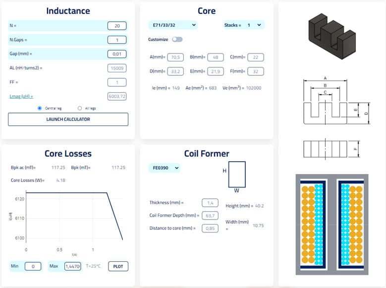
I started my design on Frenetic, deliberately choosing to start big and simple with an E71/33/32, un-gapped 3C95 core as shown in Figure 3. Using the simulator, I was able to calculate the distribution of core and copper losses between 20 kHz and 150 kHz – see Figure 4.
As the frequency increases, we can see that the core losses decrease. This is because, whilst all other parameters stay the same (or Ceteris Paribus for those who still use Latin), the increase in frequency reduces the volts-seconds imposed across the transformer primary which reduces the flux density.
Following that, when calculating the core losses, over this frequency range (and with this material) the Steinmetz coefficient for flux density has a more dominant effect on the overall equation than the coefficient for frequency. So as the frequency increase adds to the core losses, the drop in flux density has the larger net effect and therefore the core loss tends to reduce. If I was to go beyond 150 kHz and upwards, we would see the gap between the coefficients close, and the dominance of the flux density reduce. I think this is a topic for another day… Oh my.
Regarding the copper losses, the best outcome is that these losses are only caused by the DC resistance of the wires and the RMS currents through them (Irms2Rdc). As you increase the frequency however, this reality slowly fades away along with all your hopes and dreams.
So, you have on one side the core losses decreasing with frequency and on the other side the copper losses increasing. It becomes quite clear then why the intersection of these two loss mechanisms provides you with the most efficient magnetic design. For us, our magnetic here is the most efficient at around 50 kHz.
Is this the best design I could have achieved having started knowing I would use 50 kHz? I suspect I could have done a little better. But let’s continue this journey together and see where it takes us.
What happens if we change the core?
I conducted a similar analysis for two other cores E65/32/27 and E55/28/25, see the data below in Figure 5. and 6.. Before reading further though, what conclusions can you draw?
From my initial case, I have gone through three consecutive E cores reducing in size each time. I kept the number of turns the same following my rule: that I don’t particularly care about the magnetizing inductance providing it is sufficiently large. However, to make it work I have reduced the number of strands in the Litz wire to ensure there is always a comparable fit.
The first thing I notice is that the loss intersection point moves to a higher frequency as I reduce the size of the core. Why is that? Look a little deeper, you might notice that the core losses are getting higher as we reduce the size of the core and the copper losses are getting lower, so that explains why the intersection point is moving forwards.
Regarding the core losses, the only thing that I’ve changed is the effective area Ae of the core. Reducing this will increase my flux density at any given frequency. As we’ve discovered, the flux density is currently dominant for us in the core loss calculation and therefore we would expect to see an increase, this all makes sense.
Regarding the copper losses, when I reduce the size of the core, I’m also reducing the size of the window and increasing the current density. Why aren’t the copper losses increasing?
Well, I’m also reducing the amount of wire used to rap around the smaller core and therefore the DC resistance. This also has the net effect of reducing the aggressiveness of the AC resistance as we go up in frequency and overall, it softens the copper loss gradient we observe in the graphs.
I’ve managed to find an optimal operating point for a fixed transformer design using Frenetic, by simply moving the frequency around until the core and copper losses arrive at a balance. Playing with different cores whilst keeping some other parameters fixed, we saw that the optimal frequency point moved around, only on the horizontal axis though…
Headlined in the graph on Figure 7. below are the total magnetic volumes and losses I achieved over a range of frequencies, for each case I optimized my transformer and output inductor design using Frenetic Online.
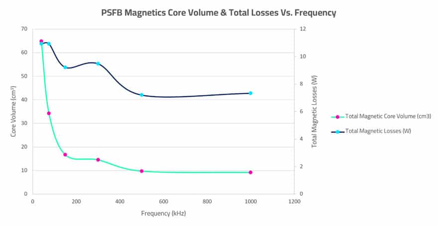
From this high-level view you can see that increasing the frequency came with its benefits. I managed to significantly reduce the volume of my Magnetics and reduce the overall losses by about 30%.
What’s not to like? Should I just keep increasing the frequency? Well, let’s look at each Magnetic in a little more detail before answering that question.
Output Inductor
Starting with the output Inductor, the first thing to mention is that I am always trying to maintain a 2Apkpk output ripple current as per the specification.
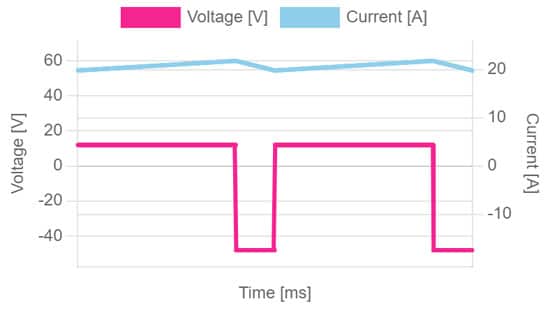
As I increase the operating frequency of the PSFB I can reduce the inductance.
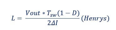
TSW is related to the operating frequency of the converter (1/FSW), but note that for this topology the ripple frequency observed by the output inductor is twice the operating frequency, hence why there is a ‘2’ is in the denominator for the equation above. There are some benefits to reducing the inductance value as we go up in frequency, and these can be explained using the formula below.
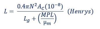
- N = Number of turns
- Ac = Effective Cross-Sectional Area of the Core, cm2
- Lg = Length of Gap, cm
- MPL = Magnetic Path Length, cm
- µm = Core Material Permeability
With the ferrite materials I used, “MPL/µm” becomes quite small, considerably more so than the length of the gap. Therefore, we effectively only have three levers we can pull to reduce our inductance value:
- Lower the cross-sectional area (smaller core).
- Reduce the number of turns (better current density).
- Increase the gap length.
During this exercise, I did none of these in isolation, in fact it was some combination of the three that led me to my optimized outcome for each design case. The volume and loss results are shown below in Figure 9., followed by my learnings.
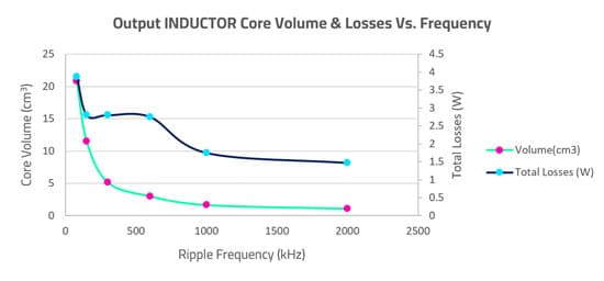
My losses could be reduced significantly – Because I was operating with only 10% as per my specification, there was very little AC ripple content and thus my core losses remained very low. At 2MHz, the core losses were at their greatest but only contributed 6% to the total losses of the inductor.
This won’t always be the case for DC Inductor designs. I chose a 10% ripple which is very conservative, and I paid the price by having a larger inductance value than I could have otherwise gotten away with. With a greater ripple content, the effects on both core losses and winding losses (from the fringing field of the gap, and proximity/skin effects) can become very significant at high frequencies. My graph above would no doubt look quite different with different ripple factors.
The AC losses in the copper remained equally small, therefore the main loss mechanism here was DC resistance of the conductor (I2R). Because I was able to both reduce the number of turns and core size with an increasing frequency, the DC resistance of the wire could reduce, thus, my losses.
- Less turns = more space, therefore thicker conductors, therefore lower resistance
- Smaller core = shorter distance to make one turn, therefore lower resistance
I could reduce the volume significantly – This is true enough, but there are some practical limits to be mindful of if I were to keep moving in this direction:
- Eventually, if the core becomes small enough or there are too few turns, the core will reach saturation.
- If, for the reason above, the turns can’t be reduced, then the current density in the windings will increase with smaller cores. Afterall, the same current is still being pushed through it, so this will begin to make cooling significantly more difficult.
- The gap size may become impractical in relation to the core size as I begin to rely on this more as a tool to manage the inductance value needed.
- The AC losses, as they eventually do, will become too significant at higher frequencies.
- Parasitic capacitances may become trickier to handle, having wider implications on the other converter elements.
- The inductor isn’t the only thing in the system, so ultimately, I’m going to need to compare the benefits that the inductor is receiving against the effects that frequency increase has on other components in the converter!
Transformer
Importantly for the transformer design, I wanted to ensure that the Converter would operate in peak current control mode, which is popular for this topology.
I used the formula below provided by a Texas Instruments App Note to calculate my required minimum transformer magnetizing inductance.
- DTYP = Duty Cycle.
- N = Turns Ratio.
- ΔILOUT = Magnitude of Output Inductor Ripple Current (2 Apkpk).
The formula used to define the duty cycle and turns ratio is as below.
You can see how for this topology it is important to minimize the leakage inductance (don’t forget you need enough to facilitate ZVS though). For us, it is going to be so much smaller than the magnetizing inductance that we can ignore it for this exercise. For simplicity, if we also assume that the diode forward voltages (Vf) are much less than the output voltage, we get a more straight-forward equation.
I fixed the duty cycle at 0.8 and the Ns/Np to 0.15, in reality I didn’t get this exactly, and it’s arbitrary but it’s a good place to start.
Hopefully now I have provided you with enough information to show that as the frequency increases, my required magnetizing inductance decreases. See below Figure 11. the evolution of my transformer designs across the range of frequencies, and some further learnings.
If I want to truly optimize, I must be willing to explore different profiles and shapes, or even customize my own core dimensions – Sticking with one core family (E Cores), as I did for the simplicity of this article, made it quite difficult to get an optimal design. The discreteness of the variables, namely turns and core dimensions, means that often the stars do not align, and one can be pushed to run with higher current densities or flux densities than desired. It’s the main reason why the graphs I have presented for both Magnetics above have bumps and notches in them.
I must understand my materials – The next problem I encountered was my reducing lack of ability to achieve the minimum magnetizing inductance I required. I made clear that I wanted to obtain a minimal magnetizing inductance, but this became harder, both as my core sizes reduced, and as I had to change my materials.
Because I didn’t change the core family (and I make a point of saying this because I haven’t done the analysis for what I’m about to say with other core shapes), as the core sizes reduced, the cross-sectional area reduced at a faster rate than the MPL. This lessened the benefits I thought I was going to get by reducing my magnetizing inductance, hence my turns count wasn’t reflected in the reduction. This meant that it became harder to maintain a manageable current density (and temperature rise).
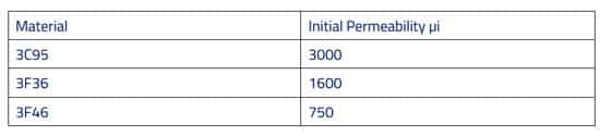
The same problem came back when I changed materials. It made sense for me as I increased the operating frequency to move from 3C95 through 3F36 to 3F46 to keep the core losses down – see Table 2. But the permeability of the materials reduced, meaning that I had to work even harder to maintain a minimum magnetizing inductance.
This is the main reason why you can see such a sharp plateau of transformer volume in the graph.
It certainly helps to understand the full picture – Finally, because there is high AC content in the waveform of the Transformer, unlike the output inductor, the AC losses are not negligible. You may notice in Figure 11 that the total losses are beginning to increase again, and this is owed to the AC resistance of the windings increasing. If I can briefly put in your mind the notions discussed in my previous Newsletter, for this experiment, with my 500 kHz design, the losses were well-balanced (44.6% Core | 55.4% Copper) meaning that I was close to the optimal efficiency of that design.
When I moved to 1MHz I ended up with the same core however, and pretty much the same number of turns for reasons I hope you will now appreciate. This meant that from the previous design, the core losses reduced, and the copper losses increased moving us further away from the optimal point (17.9% Core | 82.1% Copper). And it only goes in one direction from here.
But that doesn’t necessarily mean I have to stop increasing the frequency…
Conclusion
This all comes down to context now. I hope, if you are currently designing a PSFB that this has helped, but the extent to which my different observations affect you will vary depending on your own Converter specifications.
I observed that although moving from 500 kHz to 1 MHz didn’t give me any further volume reduction in the transformer, it also didn’t give me greatly more power losses (7.5% Increase). So perhaps I’ll be happy operating it away from its optimal frequency at 1 MHz if it means I get benefits elsewhere in the design that can justify it.
Afterall, the Inductor continued to reduce in losses and volume, and the output capacitance can reduce, further impacting my converter volume. I would finally have to trade off against the increased switching losses in my semiconductors. But with any luck I’m achieving ZVS, and this will make my job substantially easier!
The experts here at Frenetic have created powerful models, and these gave me the ability to rapidly explore my design options and understand the limitations. If you want to start making better designs, get in touch with us! And don’t forget we also have a lab with a large range of stock where we can build rapid, high-quality samples for you. We understand how important it is to get a working prototype for your converter as soon as possible so you can begin testing!