Passive Components Blog
No Result
View All Result
  • Home
  • NewsFilter
    • All
    • Aerospace & Defence
    • Antenna
    • Applications
    • Automotive
    • Capacitors
    • Circuit Protection Devices
    • electro-mechanical news
    • Filters
    • Fuses
    • Inductors
    • Industrial
    • Integrated Passives
    • inter-connect news
    • Market & Supply Chain
    • Market Insights
    • Medical
    • Modelling and Simulation
    • New Materials & Supply
    • New Technologies
    • Non-linear Passives
    • Oscillators
    • Passive Sensors News
    • Resistors
    • RF & Microwave
    • Telecommunication
    • Weekly Digest

    May 2025 Interconnect, Passives and Electromechanical Components Market Insights

    HIROSE Releases New Field-Assembly Communication Connectors

    Coilcraft Unveils 165C High-Temperature Coupled Inductors

    Bourns Releases SMD NTC Thermistors for Thermal Sensing

    Wk 22 Electronics Supply Chain Digest

    Samsung Electro-Mechanics High Capacitance MLCCs for ADAS SoCs

    Murata Expands its Automotive Common Mode Choke Coils to 150C and High Current Capability

    Bourns Releases New Current Transformer

    Skeleton Releases GrapheneGPU to Reduce AI Energy Consumption by 44% and Boosts Power by 40%

    Trending Tags

    • Ripple Current
    • RF
    • Leakage Current
    • Tantalum vs Ceramic
    • Snubber
    • Low ESR
    • Feedthrough
    • Derating
    • Dielectric Constant
    • New Products
    • Market Reports
  • VideoFilter
    • All
    • Antenna videos
    • Capacitor videos
    • Circuit Protection Video
    • Filter videos
    • Fuse videos
    • Inductor videos
    • Inter-Connect Video
    • Non-linear passives videos
    • Oscillator videos
    • Passive sensors videos
    • Resistor videos

    Coupled Inductors Circuit Model and Examples of its Applications

    Inductor Resonances and its Impact to EMI

    Highly Reliable Flex Rigid PCBs, Würth Elektronik Webinar

    Causes of Oscillations in Flyback Converters

    How to design a 60W Flyback Transformer

    Modeling and Simulation of Leakage Inductance

    Power Inductor Considerations for AI High Power Computing – Vishay Video

    Coupled Inductors in Multiphase Boost Converters

    VPG Demonstrates Precision Resistor in Cryogenic Conditions

    Trending Tags

    • Capacitors explained
    • Inductors explained
    • Resistors explained
    • Filters explained
    • Application Video Guidelines
    • EMC
    • New Products
    • Ripple Current
    • Simulation
    • Tantalum vs Ceramic
  • Knowledge Blog
  • Suppliers
    • Who is Who
  • Events
No Result
View All Result
Passive Components Blog
No Result
View All Result

LTspice Worst-Case Circuit Analysis with Non-Ideal Resistors at Minimal Simulations Runs

24.8.2022
Reading Time: 8 mins read
A A

When designing a circuit in LTspice, you may wish to assess the impact of component tolerances. For example, the gain error introduced by non-ideal resistors in an op amp circuit. This article written by Gabino Alonso and Joseph Spencer from Analog Devices illustrates a method that reduces the number of simulations needed, and as a result speeds your time to results.

Varying a Parameter

RelatedPosts

May 2025 Interconnect, Passives and Electromechanical Components Market Insights

HIROSE Releases New Field-Assembly Communication Connectors

Coilcraft Unveils 165C High-Temperature Coupled Inductors

LTSpice provides several ways to vary the value of a parameter. Some of these are:

  • .step param; A parameter sweep of a user-defined variable
  • gauss(x); A random number from Gaussian distribution with a sigma of x
  • flat(x); A random number between -x and x with uniform distribution
  • mc(x,y); A random number between x*(1+y) and x*(1-y) with uniform distribution.

These functions are very useful, especially if we want to look at results in terms of a distribution. But if we only want to look at worst case conditions, they may not be the quickest way to get a result. Using gauss(x), flat(x) and mc(x,y) for example, will require a simulation to run for a statistically significant number of times. From there, a distribution can be looked at and worst case values calculated in terms of standard deviations. However, for a worst case analysis we would prefer not to use a distribution approach, instead the maximum deviation from the nominal value of each component are used in the calculations.

Running Minimal Simulations

Let’s say that we want to look at the worst-case impact of a R1 = 22.5kΩ resistor with a 1% tolerance. In this case, we really only want to run the simulation with R1 = 22.5kΩ * (1 – 0.01) and 22.5kΩ * (1 + 0.01). A third run with an ideal 22.5kΩ resistor would also be handy to have.

.step param R1 list 22.5k*(1-.01) 22.5k*(1+.01) 22.5k

If we were just varying one resistor value, the ‘.step param’ method would work very well. But what if we have more? The classic difference amplifier has 4 resistors.

LTspiceWCA_Figure_1
Figure 1. Difference Amplifier Configuration (From the LT1997-3 datasheet)

If a discrete difference amplifier were to be designed, each of these would have some tolerance (e.g. 1% or 5%).

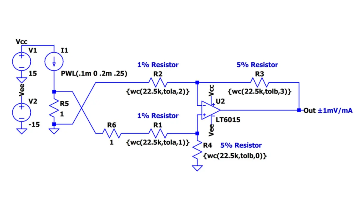
For an example, let’s take the front page application shown in the LT1997-3 datasheet and implement it in LTspice with a discrete LT6015 op-amp and some non-ideal resistors.

LTspiceWCA_Figure_2
Figure 2. LT1997-3 Front Page Application Example
LTspiceWCA_Figure_3
Figure 3. LT6015 Difference Amplifier with Non-Ideal Resistors

Notice the values of resistors R1, R2, R3 and R4 are replaced by a function call wc(nominalvalue, tolerance, index) which is defined in the simulation by a .func statement:

.func wc(nom,tol,index) if(run==numruns,nom,if(binary(run,index),nom*(1+tol),nom*(1-tol)))

This function in conjunction with the binary(run, index) function below vary the parameter for each component between its maximum value and minimum values and for the last run the nominal value.

.func binary(run,index) floor(run/(2**index))-2*floor(run/(2**(index+1)))

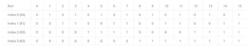
The binary function toggles each index’ed componment in the simulation so that all possible combination of nom*(1+tol) and nom*(1-tol) are simulated. Note that the index of components should start with 0. The following table highlights the operation of the binary() function with results to each index and run, where 1 represents nom*(1+tol) and 0 represents nom*(1-tol).

The number of runs is determined buy 2N +1, where N equals the number of indexed components, to cover all the max and min combinations of the device plus the nominal. In our case we need 17 simulations run and we can define this using the .step command and the .param statments:

.step param run 0 16 1
.param numruns=16

Lastly, we need to define the tola and tolb for the simulation via .param statments:

.param tola=.01
.param tolb=.05

You can find more information about the .func, .step, and .param statments in the help (F1) and under the .param section details about the if(x,y,z) and floor(x) functions.

Plotting the .Step’ed Results

If the transient analysis simulation is run, see WorstCase_LT6015.asc file, we can observe our results. For a 250mA test current, we expect the Vout net to settle to 250mV. But now with our wc() function, we get a spread from 235mV to 265mV.

LTspiceWCA_Figure_4
Figure 4. Difference Amplifier Transient Analysis

Plotting the .Step’ed .Meas Statement

At this point we could zoom in and look at the peak to peak spread. But let’s take a lesson from another LTspice blog:

Plotting a Parameter Against Something Other Than Time (e.g. Resistance)

This blog covers how to run a simulation several times and plot a parameter against something other than time. In this case, we want to plot the V(out) vs. simulation run index. See WorstCase_LT6015_meas.asc file.

In this simulation we have add a .meas statment to calculated the average voltage of the output.

.meas VoutAvg avg V(out)

To plot the V(out) vs. run parameter we can view the SPICE Error Log (Ctrl-L), right click and select Plot .step’ed .meas data.

LTspiceWCA_Figure_5
Figure 5. Spice Error Log Interface

The plot results of our .step‘ed .meas data.

LTspiceWCA_Figure_6
Figure 6. Output Voltage vs. Simulation Run

The trace hows us that the results vary from a maximum worse case of 265mV (run 9) to a minimum worse case of 235mV (run 6) or roughly a ±6% error. This makes some intuitive sense since we had both 1% and 5% resistors in this example. The last run (16) shows the ideal result (250mV) which is ideal resistors. Recall LTspice graphs the results from the .meas statment as a piece wise linear graph.

Another faster approach to this particular circuit is to use the .op simulation (instead of the .trans) to perform a DC operating point solution which will plot the results of our stepped.meas data directly.

The Value of Matched Resistors

When designing a difference amplifier not only is the appropriate op-amp needed, but equally as important are the matching of the resistors. The following references do an excellent job of explaining this topic (and associated math) in detail:

  • LT5400 (Quad Matched Resistor Network) Datasheet
  • Design Note DN1023
  • Design Note DN502

However, you can neither achieve good Common Mode Rejection Ratio (CMRR) or Gain Error without appropriately matched resistors.

Linear Technology, now part of Analog Devices, has a number of precision amplifier products which also include matched resistors. A recently released example of this is the LT1997-3 – Precision, Wide Voltage Range Gain Selectable Amplifier. Two key specifications are:

  • 91dB Minimum DC CMRR (Gain = 1)
  • 0.006% (60ppm) Maximum Gain Error (Gain = 1)

These specifications are really quite excellent. According to DN1023, CMRR due only to 1% resistors (with an ideal op-amp) will limit your CMRR to 34dB. And of course, the gain error is orders of magnitude worse than what the LT1997-3 achieves.

Summary

Using the method outlined above, a simple worst-case analysis can be run at the min/max value of several parameters. In this example we looked at the impact of resistor tolerances in a classical difference amplifier, and the value of the matched resistors in the LT1997-3 are illustrated.

References

Monte Carlo and Worst-Case Circuit Analysis using LTSpice

Related

Source: Analog Devices

Recent Posts

Coupled Inductors Circuit Model and Examples of its Applications

21.5.2025
89

Würth Elektronik Introduces LTspice Models for ESD Products

21.5.2025
50

Littelfuse Gate Driver Integrates Diode and Current Limit Resistor in Compact IC

21.5.2025
22

Capacitor Ripple Current Testing: A Design Consideration

21.5.2025
75

Inductor Resonances and its Impact to EMI

16.5.2025
78

Causes of Oscillations in Flyback Converters

15.5.2025
46

Vishay Releases Automotive SMD Thick Film Power Resistor for Enhanced Protection Against Short Transient Pulses

14.5.2025
20

How to design a 60W Flyback Transformer

12.5.2025
70

Bourns Extends Rotational Life Option for its Guitar Potentiometer

9.5.2025
13

Modeling and Simulation of Leakage Inductance

9.5.2025
45

Upcoming Events

Jun 4
11:00 - 12:00 CEST

Würth Elektronik PCB Production in Asia

Jun 24
17:00 - 18:00 CEST

Ultra-Compact and Efficient Switched-Capacitor Power Converters

View Calendar

Popular Posts

  • Buck Converter Design and Calculation

    0 shares
    Share 0 Tweet 0
  • Flyback Converter Design and Calculation

    0 shares
    Share 0 Tweet 0
  • Boost Converter Design and Calculation

    0 shares
    Share 0 Tweet 0
  • LLC Resonant Converter Design and Calculation

    0 shares
    Share 0 Tweet 0
  • What is a Dielectric Constant and DF of Plastic Materials?

    4 shares
    Share 4 Tweet 0
  • What Electronics Engineer Needs to Know About Passive Low Pass Filters

    0 shares
    Share 0 Tweet 0
  • Dual Active Bridge (DAB) Topology Explained

    0 shares
    Share 0 Tweet 0
  • Wk 22 Electronics Supply Chain Digest

    0 shares
    Share 0 Tweet 0
  • How to Design an Inductor

    0 shares
    Share 0 Tweet 0
  • Coefficient of Linear Thermal Expansion on Polymers Explained

    0 shares
    Share 0 Tweet 0

Newsletter Subscription


Passive Components Blog

© EPCI - Leading Passive Components Educational and Information Site

  • Home
  • Privacy Policy
  • EPCI Membership & Advertisement
  • About

No Result
View All Result
  • Home
  • Knowledge Blog
  • Premium Suppliers

© EPCI - Leading Passive Components Educational and Information Site

This website uses cookies. By continuing to use this website you are giving consent to cookies being used. Visit our Privacy and Cookie Policy.
Go to mobile version