


This article and video presentation by Sam Ben-Yaakov challenge conventional wisdom and reveal that the widely recommended method of adding a parallel resistor across the thermistor doesn’t actually enhance linearity when evaluated accurately. Instead, it diminishes sensitivity and creates a deceptive visual improvement in plots that aren’t normalized for span.
Key Takeaways
- Sam Ben-Yaakov’s article challenges the idea that adding a parallel resistor across a thermistor improves linearity; it actually reduces sensitivity.
- The NTC thermistor has a non-linear resistance-temperature relationship, complicating accurate measurements when using a voltage divider.
- Popular methods for linearizing thermistor output do not deliver true linearity; the apparent improvement with a parallel resistor is misleading.
- Simulation results confirm that using a parallel resistor decreases sensitivity without enhancing linearity, as revealed through Thevenin equivalent analysis.
- For better accuracy, designers should focus on optimizing a single series resistor and consider digital linearization techniques for thermistors.
Introduction
NTC thermistors are widely used for temperature sensing thanks to their high sensitivity, low cost and simple interface with standard analog circuits and ADCs.
Despite these advantages, the strongly non-linear resistance–temperature characteristic complicates accurate measurement when a simple voltage divider is used. A popular “analog linearization” technique is to add a fixed resistor either in series or in parallel with the thermistor in order to obtain a more linear voltage–temperature response over a limited range.
Role of thermistor linearization in practice
NTC thermistors are widely used in power supplies, battery packs, HVAC controllers, EV chargers and industrial sensors, where they provide affordable temperature monitoring and protection over spans from roughly −40 °C to +150 °C. In these systems, linearization is often introduced to keep the output within ADC range, simplify calibration and achieve acceptable accuracy without over‑specifying the microcontroller or reference circuitry. Understanding what linearization can and cannot achieve is therefore crucial for designing robust and cost‑effective temperature‑sensing front‑ends.
Core Concepts of Thermistor Linearization
NTC thermistor characteristics
Negative Temperature Coefficient (NTC) thermistors exhibit a resistance that decreases rapidly with increasing temperature, often modeled by an exponential or Steinhart–Hart-type relationship over the operating range:
For many power electronics and general sensing applications, the relevant temperature span is roughly from −40 °C to +150 °C, within which the resistance can change by an order of magnitude or more. The high sensitivity (large dR/dT) makes NTC thermistors attractive for ADC-based measurement, but the associated non-linearity means that a direct voltage divider output is far from linear in temperature.
Common analytical models
A frequently used simplified model for an NTC thermistor relates resistance R(T) at temperature T to a reference resistance Rref at Tref using an exponential law equivalent to a truncated Steinhart–Hart expression. Manufacturers often provide either explicit Steinhart–Hart coefficients or compact exponential fits, and many also supply ready-to-use SPICE macro-models that realize the non-linear resistance in simulation. Such models are accurate enough across the typical operating interval to evaluate linearization strategies quantitatively.
Overview of linearization options
Before comparing specific resistor networks, it is useful to distinguish the main categories of thermistor linearization used in practice. Each approach involves a trade‑off between accuracy, component count, flexibility and ease of calibration.
- Simple series divider (analog) – The thermistor forms a divider with a single fixed resistor, with the output taken across either element. Linearity is locally optimized around a chosen midpoint temperature, and performance over a wider span depends heavily on the chosen series resistance.
- Series plus parallel resistor (analog) – A fixed resistor is added in parallel with the thermistor while retaining the series resistor, with the goal of “straightening” the voltage–temperature curve. In reality this configuration mainly reduces the effective resistance swing and output span and, when evaluated with normalized metrics, does not significantly improve linearity compared to a well‑chosen series‑only divider.
- Advanced analog shaping networks – Additional diodes, transistors or segmented resistor networks are used to approximate the thermistor’s exponential behavior with piecewise linear segments. These circuits can improve linearity over a defined range but at the cost of higher component count, more complex design and limited flexibility if the sensing range or thermistor type changes.
- Digital linearization with equations – The thermistor divider output is digitized and the resistance–temperature relationship is inverted in firmware using the Steinhart–Hart equation or an exponential model fitted to the datasheet. With adequate ADC resolution and calibration, this method can achieve sub‑degree accuracy over wide temperature spans without complex analog networks.
- Digital linearization with lookup tables – Pre‑computed tables map ADC codes to temperature, optionally with interpolation, making it easy to correct residual non‑linearity and manufacturing spread. This is especially effective when combined with production calibration and is generally the preferred option in modern microcontroller‑based systems.
Classical Linearization Approaches
Series-resistor method
The simplest configuration uses the thermistor RT in series with a fixed resistor RS driven from a reference voltage, with the output taken across the thermistor (or across the resistor, depending on polarity preference). A widely taught rule of thumb states that for best “local linearity” around a chosen temperature T0, the series resistor should be selected approximately equal to the thermistor resistance at that temperature, i.e. RS ≈ RT(T0). This configuration yields a reasonably linear response only within a relatively narrow temperature band surrounding T0, and becomes increasingly non-linear as the temperature deviates from that point.
Parallel-resistor “improvement” method
To extend the apparently linear region, many application notes propose adding a fixed resistor RP in parallel with the thermistor, while still using a series resistor RS to form the voltage divider. Published design recipes provide closed-form expressions or graphical methods to select RS and RP given a nominal resistance at a reference temperature and a target measurement range, and they typically present plots where the output curve with RP appears visually closer to a straight line. This visual impression has encouraged the belief that the parallel resistor genuinely improves linearity over the same measurement span.
Revealing the Linearization Misconception
Voltage span versus linearity metric
A crucial observation is that many “before and after” plots compare a full-span response without the parallel resistor (for example, output varying from near 0 V to near the supply voltage) to a much narrower-span response when RP is added. With the thermistor shunted, the effective resistance range shrinks and the output voltage swing across the temperature range of interest may be reduced from, say, 10 V to 3 V, which naturally compresses deviations from an ideal straight line when viewed on the same absolute vertical scale. This creates an illusion of improved linearity, even though the ratio of deviation to total span (and therefore the effective nonlinearity in V/°C) has not necessarily improved.
Using a normalized linearity criterion
To assess linearity meaningfully, the deviation from a best-fit straight line must be considered relative to the overall sensitivity, typically characterized as volts per degree Celsius, not just in absolute voltage units. When the output curves are scaled to the same span (for example, by dividing the “no parallel resistor” curve by an appropriate factor so that both responses cover the same vertical range), the apparent advantage of the parallel resistor disappears and the two curves exhibit essentially the same shape of non-linearity. In other words, the parallel resistor has merely reduced sensitivity rather than improving the intrinsic linear relationship between temperature and output voltage.
Thevenin-Based Circuit Interpretation
Equivalent circuit derivation
Consider the standard configuration with a supply voltage, a series resistor RS, and the thermistor RT(T) in parallel with a fixed resistor RP, with the output taken at the junction. By “cutting” the circuit at the output node and replacing the source plus series resistor network with its Thevenin equivalent as seen from that node, one can show that the series–parallel arrangement is equivalent to a single effective series resistor plus a Thevenin voltage source. The parallel network of RS and RP can be collapsed into one resistance, and the voltage division between them yields a fixed Thevenin source that subtracts from the original supply as seen by the thermistor.
Impact on effective excitation and sensitivity
In this Thevenin view, the thermistor is still driven by a series resistance, but now the effective excitation voltage is reduced because part of the supply is dropped across the internal Thevenin source in the opposite direction. Since the linearity of the voltage–temperature transfer is governed by the interaction between the thermistor’s non-linear resistance and the single series resistance, the presence of a fixed offset source does not change the non-linear functional shape; it only shifts and scales the response. As a result, the circuit with a parallel resistor yields essentially the same normalized non-linearity as a single appropriately chosen series resistor, but with lower overall sensitivity (smaller volts-per-degree span).
Simulation-Based Evidence
LTspice test setup
To quantify these effects, a non-linear resistor model representing the NTC thermistor is implemented in LTspice using an expression that encodes the exponential resistance–temperature relationship, fitted to manufacturer data at a reference resistance R25 (for example, 10 kΩ at 25 °C). A transient simulation sweeps a “temperature” control variable from −40 °C to +150 °C using a ramp source, and the output voltage across the thermistor is recorded together with its temperature derivative to obtain sensitivity in volts per degree (with optional scaling for convenient plotting). Multiple subcircuits are instantiated: one with only a series resistor, one with an additional parallel resistor of a value borrowed from a published example, the corresponding Thevenin-equivalent circuit, and a variant where the Thevenin source is removed but the equivalent resistance is kept.
Results and interpretation
The simulation shows that the “series plus parallel” and its exact Thevenin-equivalent circuit produce identical output and sensitivity curves, as expected from linear circuit theory. When comparing the series-only configuration to the series-plus-parallel configuration, the latter exhibits a much smaller output span and significantly reduced sensitivity, even though its curve may look slightly “flatter” on an absolute scale. After scaling the high-span series-only response down by the same factor by which the Thevenin offset reduces the effective voltage, the normalized curves overlap closely, demonstrating that the parallel resistor has not improved the intrinsic linearity, only sacrificed sensitivity.
Simple numeric illustration
To make the effect more concrete, consider a 10 kΩ NTC at 25 °C with a β value typical for general‑purpose sensing, biased from a fixed reference in two configurations: a series‑only divider and a series‑plus‑parallel network chosen according to a published example. The values below are illustrative, but they capture the qualitative behavior seen in detailed LTspice simulations.
| Temperature | Series-only: output (V) | Series + parallel: output (V) | Normalized deviation comparison |
|---|---|---|---|
| −20 °C | Higher absolute voltage; large span from cold to hot | Lower absolute voltage; total span compressed by shunting | Apparent error looks larger in absolute volts for the series‑only case, but similar when expressed as a percentage of span |
| 25 °C | Midpoint of range; series resistor chosen near RT(25 °C) for best local linearity | Operating point shifted and scaled due to Thevenin offset produced by the parallel branch | Both configurations show comparable normalized deviation around the midpoint |
| 80 °C | Lower output than at 25 °C; still substantial voltage swing per degree | Output reduced and sensitivity flattened because part of the current bypasses the thermistor | Normalized deviation versus best‑fit line remains similar between the two networks |
Practical Design Implications
Why the parallel resistor method persists
The popularity of the parallel resistor method likely stems from design flows where the initial choice of series resistor is suboptimal; adding a parallel resistor then “trims” the effective resistance seen by the thermistor and incidentally brings the operating point closer to an optimum. Because many published plots omit normalization and show only absolute voltages, this trimming effect can be misinterpreted as a fundamental linearization improvement attributable to the parallel branch itself. In reality, an equivalent or better result could be achieved by simply adjusting the series resistor alone, without the undesirable reduction in sensitivity and without introducing a DC offset through the Thevenin source.
Recommended analog front-end strategy
For analog front‑ends that still rely on a simple divider, a structured design process helps to avoid the pitfalls associated with the parallel resistor method. The following checklist summarizes a practical workflow that can be implemented quickly using a circuit simulator or numerical tools.
- Define the temperature range and accuracy budget.
- Specify minimum and maximum temperatures (for example −40 °C to +150 °C) and decide how much of the total error budget may be allocated to linearization, as opposed to sensor tolerance, self‑heating or ADC errors.
- Select the thermistor and obtain a suitable model.
- Choose an NTC with appropriate nominal resistance and β value, and obtain Steinhart–Hart coefficients, an exponential fit or a SPICE macro‑model from the manufacturer.
- Simulate a simple series divider.
- Connect the thermistor in series with a single resistor and the reference voltage, sweep temperature across the full range, and record both the output voltage and volts‑per‑degree sensitivity.
- Optimize the single series resistor.
- Adjust the series resistor value, starting near RT at the midpoint temperature, to maximize sensitivity while minimizing normalized deviation from a best‑fit straight line over the desired span.
- Avoid using a parallel resistor for linearization.
- Do not add a parallel resistor solely to “straighten” the curve, because it mainly compresses the output span and introduces a Thevenin offset without materially improving normalized linearity.
- Use attenuation or scaling only when necessary.
- If the optimized divider produces a voltage span that is too large for the ADC, add an explicit attenuator or adjust the reference voltage instead of re‑tuning the thermistor network to act as a hidden attenuator.
- Plan for digital linearization.
- Where possible, convert measured voltage to resistance and temperature in firmware using Steinhart–Hart or a calibrated lookup table, which can correct the residual non‑linearity and absorb part‑to‑part tolerance.
Linearization in the overall error budget
In many practical systems, the dominant error sources are thermistor tolerance at the reference temperature, β coefficient spread, self‑heating and ADC reference uncertainty rather than the residual non‑linearity of a well‑designed divider. Once digital correction is available, the remaining impact of analog linearization techniques often becomes secondary, so it is generally more effective to invest effort in calibration and error budgeting than in adding extra resistors around the thermistor.
Alternative Approaches to Linearity
Digital linearization
In modern designs, the most robust and accurate way to handle thermistor non-linearity is to digitize the divider voltage directly and apply either the full Steinhart–Hart equation or a high-resolution lookup table in firmware. With adequate ADC resolution, calibration data and computational resources, this approach can linearize the response to within fractions of a degree over wide temperature spans, making purely analog linearization networks unnecessary except in legacy or ultra-low-cost designs.
Alternative analog techniques
Where digital post-processing is not feasible, more sophisticated analog approaches—such as using complementary non-linear elements, transistor-based shaping networks or multi-segment piecewise-linear approximations—can be employed to better match the thermistor’s exponential behavior. However, these solutions add complexity and component count, and for most practical systems the combination of a well-optimized simple divider and digital correction provides a superior trade-off between accuracy, flexibility and cost.
Illustrative Design Data
Example parameter table
Table 1 summarizes an illustrative comparison between a “series-only” and a “series plus parallel” configuration over a nominal −40 °C to +150 °C range, based on the qualitative trends reported in the reference analysis. Exact numeric values depend on the particular thermistor and resistor choices, but the relative trends are generic.
| Metric | Series-only divider | Series + parallel resistor |
|---|---|---|
| Output span over −40 °C to +150 °C | Large span (for example from near 0 V to near the supply voltage) | Much smaller span (often only about 30–40 % of the supply voltage) |
| Sensitivity (V/°C) | High sensitivity due to large output span | Significantly reduced sensitivity because the thermistor swing is shunted by the parallel resistor |
| Apparent deviation from straight line (absolute volts) | Visibly larger on unnormalized plots because the full span is shown | Visibly smaller absolute error, but largely due to the compressed vertical scale |
| Normalized deviation (relative to span) | Comparable to the series‑plus‑parallel case after scaling to the same span | Comparable to the series‑only case when evaluated with a proper normalized linearity metric |
| DC offset / operating point shift | No additional DC offset beyond the basic divider behavior | Introduces an effective DC offset via the Thevenin equivalent source |
| Component count and complexity | One resistor plus thermistor, minimal design complexity | Two resistors plus thermistor, extra design steps and more chances for misinterpretation |
| Approach | Pros | Limitations |
|---|---|---|
| Optimized series divider only | Lowest component count, easy to simulate, good enough for many protection and monitoring tasks | Limited linearity over wide spans, residual error must be tolerated or corrected elsewhere |
| Divider plus digital linearization | High accuracy over wide temperature ranges, easy to adapt in firmware, can absorb part‑to‑part spread via calibration | Requires ADC resolution and firmware resources, design effort shifts to software and data management |
Conclusion
The analysis of thermistor linearization networks shows that adding a fixed parallel resistor across an NTC thermistor in a divider does not intrinsically improve linearity when performance is judged using a normalized metric such as deviation relative to volts-per-degree sensitivity.
Interpreted through Thevenin equivalence and confirmed in LTspice simulations, the series-plus-parallel configuration is effectively equivalent to a single series resistor driven from a reduced excitation voltage, leading primarily to a loss of sensitivity rather than an improvement in transfer linearity.
For analog thermistor front-ends, designers are therefore encouraged to optimize a single series resistor (optionally followed by simple attenuation if necessary) and, where possible, to rely on digital linearization—via Steinhart–Hart or lookup tables—to achieve high accuracy over wide temperature ranges.
Yoast FAQ: Thermistor Linearization Challenges
A parallel resistor remains useful when the primary goal is to limit the maximum resistance or voltage at extreme temperatures, or to constrain the overall span for protection or biasing purposes. In such cases it acts as a deliberate attenuator or clamp, but it should not be regarded as a genuine linearization element because the normalized non‑linearity of the thermistor response is largely unchanged compared to an optimized series‑only divider.
Yes, many modern microcontroller systems simply read the raw divider output from a basic series network and perform all linearization digitally using equations or lookup tables. Provided that the ADC input range and resolution are adequate, and the firmware correctly implements the thermistor model and calibration data, this approach can deliver better accuracy and flexibility than more complex analog linearization networks.
The main message is that adding a fixed parallel resistor across an NTC thermistor in a voltage divider does not truly improve the linearity of the temperature–voltage transfer; it primarily reduces the signal span and sensitivity, while the normalized non-linearity remains essentially unchanged compared to an optimized series-only resistor configuration.
Many application notes and examples present plots where the configuration with a parallel resistor shows a smaller absolute deviation from a straight line, but these plots usually compare a narrow-span response to a much larger-span response, creating a visual illusion of better linearity because the vertical scale is compressed.
Linearity should be evaluated using a normalized metric such as deviation from a best-fit straight line relative to the volts-per-degree sensitivity, rather than absolute voltage error, and when curves are normalized to the same span, the supposed advantage of the parallel resistor disappears.
The Thevenin equivalent shows that the series-plus-parallel network is functionally equivalent to a single series resistor driven by a reduced effective excitation voltage, so the non-linear shape of the thermistor’s response remains the same while the output span and sensitivity are simply scaled down.
The article recommends selecting and optimizing a single series resistor for the desired temperature range using simulation, avoiding the use of a parallel resistor purely for linearization, and adding a separate attenuator only if the reduced span is explicitly required by the ADC or interface.
By digitizing the divider voltage and applying the Steinhart–Hart equation or a lookup table in firmware, designers can achieve high accuracy and effective linearization over wide temperature ranges, often making complex analog linearization networks unnecessary.
How-to Best Achieve Linearization of a NTC Thermistor
- Define the temperature range and resolution requirements
Start by specifying the minimum and maximum temperatures to be measured, such as −40 °C to +150 °C, and determine the required resolution and accuracy in degrees Celsius for your application.
- Select an appropriate NTC thermistor and obtain its model
Choose a thermistor with a suitable nominal resistance (for example 10 kΩ at 25 °C) and operating range, and obtain its Steinhart–Hart coefficients, exponential fit or SPICE macro-model from the manufacturer’s datasheet.[
- Build a basic series resistor divider in simulation
In a circuit simulator such as LTspice, connect the thermistor in series with a fixed resistor and a reference voltage source, then sweep the temperature from the minimum to maximum values while recording the divider output voltage and its derivative with respect to temperature.
- Optimize the single series resistor for linearity and sensitivity
Adjust the series resistor value, starting near the thermistor resistance at the midpoint temperature, to maximize volts-per-degree sensitivity while minimizing the normalized deviation from a best-fit straight line over the chosen temperature span.
- Avoid adding a parallel resistor for linearization
Do not rely on a parallel resistor to the thermistor as a linearization element, because it mainly compresses the output span and reduces sensitivity without significantly improving the normalized linearity compared to a well-chosen single series resistor.
- Use attenuation or scaling only when necessary
If the optimized divider produces a voltage span that exceeds the ADC input range, add a simple attenuator or adjust the reference voltage rather than modifying the thermistor network in ways that obscure the linearity behavior.
- Implement digital linearization in firmware
Convert the measured voltage to resistance and then to temperature using the Steinhart–Hart equation or a calibrated lookup table in firmware to achieve accurate, repeatable linearization across the full operating temperature range.
- Validate the design with measurements
Finally, build a prototype, measure the output at multiple known temperatures, and compare the results to the simulated and calculated values to confirm that the optimized single-resistor design meets your accuracy and sensitivity targets.