Advanced Loss Modeling for Planar Magnetics in the Frenetic Planar Tool

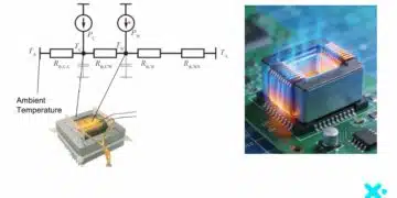
Planar magnetics promise compact, low‑profile magnetics, but accurate loss, leakage, and capacitance modeling is significantly more complex than for conventional wound components.

This paper based on Frenetic webinar explains the modeling strategy behind the Frenetic planar tool, combining analytical methods with finite element simulations and a quasi‑3D approach.

Engineers gain a precise workflow for designing planar transformers and inductors, including loss separation, leakage tuning via interleaving, capacitance estimation, and gap optimization. The paper also proposes practical tables and visualization concepts to turn these models and demo results into actionable design data for deployment in real power converters.

Introduction

Planar transformers and inductors are increasingly used in high‑density power electronics, especially where strict profile constraints and automated PCB assembly are key requirements. While planar windings offer repeatable geometry, good thermal behavior, and excellent scalability, they introduce strong eddy current effects and elevated parasitic capacitances compared to traditional round‑wire magnetics. These phenomena can dramatically change AC losses, leakage inductance, and resonant behavior, and they cannot be captured by simple extensions of conventional models.

The Frenetic planar tool has been developed to address these challenges by combining a finite element method (FEM) core with advanced analytical post‑processing and a dedicated quasi‑3D transformation. Its purpose is to provide accurate planar loss and parasitic models directly usable by power and magnetics designers, while keeping simulation time compatible with iterative design workflows. This paper outlines the underlying modeling approach and shows, through a flyback converter case, how engineers can integrate the planar tool into a complete design flow, from initial AI‑based magnetics suggestions to detailed planar PCB layout and parasitic fine‑tuning.

Background and Challenge

Conventional magnetics loss modeling in Frenetic’s simulator starts from solid round conductors wound around a magnetic core and including one or more air gaps. For such geometries, proximity losses can be accurately computed using analytical methods once the current distribution and magnetic field in the winding window are known. The standard workflow is:

1. Represent the air gap as an equivalent fictitious current source that reproduces the fringing field of the gap.
2. Remove the magnetic material by replacing it with mirrored equivalent current sources (method of images), maintaining the same field in the window.
3. Reduce the problem to a plane populated by many equivalent conductors and compute the magnetic field in each conductor as the superposition of contributions from all others.

This approach works well for round wires because induced eddy currents remain relatively small and do not significantly distort the magnetic field distribution. Once the current through a conductor and the magnetic field it experiences are known, skin and proximity losses can be calculated with established analytical expressions.

In planar PCB windings, however, conductor geometry changes radically: traces are thin in height and wide in width, leading to a large width‑to‑thickness aspect ratio. When the magnetic field has a component orthogonal to the trace surface, very strong eddy currents are induced within the copper. These eddy currents can become large enough to distort the magnetic field itself, breaking the assumptions on which the conventional proximity‑loss model relies. For planar magnetics, this feedback between eddy currents and local field cannot be neglected, so the previous modeling approach becomes inaccurate.

At the same time, planar cores and PCB windings naturally yield higher parasitic capacitances, especially between primary and secondary layers and between turns within a winding. These capacitances strongly influence the first resonant frequency of the structure and thus define the upper frequency limit for reliable operation. Any accurate planar modeling framework therefore needs to consider both advanced loss mechanisms and detailed capacitance extraction, while still providing leakage inductance estimates compatible with converter‑level simulations.

Key Technical Concepts

• Fictitious gap current: The air gap of a magnetic core is replaced by an equivalent current source whose magnitude equals the magnetic flux times the gap reluctance, reproducing the fringing field in the winding window.
• Method of images: Magnetic material is removed and replaced by mirrored current sources such that the field in the winding region remains unchanged, enabling an equivalent “plane of conductors” representation.
• Proximity loss calculation: Once conductor current and local magnetic field are known, proximity and skin effect losses are obtained via analytical expressions, which are reliable for round conductors but insufficient for planar traces.
• Planar eddy current distortion: Thin, wide PCB traces subjected to fields with orthogonal components experience strong eddy currents that significantly distort the magnetic field and invalidate simplified proximity models.
• Finite Element Method (FEM) engine: A 2D FEM model, implemented in Comsol and solved in the cloud, directly solves Maxwell’s equations for the given geometry, capturing all relevant physical effects including skin and proximity losses and interactions among parallel windings.
• Quasi‑3D modeling: Results from 2D FEM slices are transformed into effective 3D quantities using a quasi‑3D concept that adjusts the effective turn length and localizes losses according to where they physically occur along the winding path.
• Capacitance modeling: Planar structures include a primary open‑circuit capacitance model that allows estimation of the first resonant frequency when combined with primary inductance, defining the feasible frequency range.
• Analytical leakage model: Leakage inductance is still computed analytically within the planar tool, enabling fast evaluation of interleaving strategies and auxiliary winding placement without needing full FEM for every iteration.
• Harmonic‑resolved loss computation: The tool can import winding waveforms in CSV format and consider multiple harmonics (DC, fundamental, higher odd components) to calculate losses under realistic excitation.
• Iterative planar layout refinement: Engineers can adjust layer count, turn distribution, spacing, and interleaving to trade off current density, leakage inductance, and losses, with FEM providing quantitative feedback.

Analysis and Implementation

Overall Modeling Architecture

The Frenetic planar tool integrates three primary models within its architecture: a FEM‑based loss model, a parasitic capacitance model, and an analytical leakage inductance model. Engineers access these models through an application that defines the transformer or inductor geometry, generates appropriate mesh and boundary conditions, triggers simulations, and returns processed quantities such as DC and AC losses, leakage inductances between windings, and open‑circuit capacitances.

The modeling pipeline can be summarized as:

1. Geometry and parameter definition in the planar app (core type, gaps, PCB window, windings, currents).
2. Conversion of geometry into a 2D FEM model in Comsol and generation of a magnetic mesh.
3. Application of boundary conditions and interconnections corresponding to excitation waveforms for each winding.
4. Numerical solution of Maxwell’s equations to obtain field distributions and local loss densities.
5. Quasi‑3D transformation of 2D results into 3D loss and inductance values.
6. Analytical computation of leakage inductances and selected capacitances.
7. Post‑processing and return of total losses per winding, leakage matrix entries, and key capacitances to the planar app.

This framework allows the tool to capture complex interactions within planar structures while maintaining an interactive design experience, with typical FEM calculations requiring on the order of 20–40 seconds per configuration.

Conventional Loss Modeling and Its Limitations

In the conventional (non‑planar) Frenetic simulator, losses are calculated by representing the core and gap using equivalent currents and a mirroring method. The air gap is replaced by a fictitious current whose magnitude is:$$I_{\text{mag}} = \Phi \, \mathcal{R}_{\text{gap}}$$where $\Phi$ is the magnetic flux and $\mathcal{R}_{\text{gap}}$ is the reluctance of the gap. This current reproduces the same magnetic field as the original gap region in the surrounding space.

Next, the magnetic material is removed from the model and replaced by mirrored current sources. The objective is to preserve the magnetic field in the winding window while simplifying the geometry. After sufficient mirroring iterations, the configuration resembles an infinite plane populated with conductors (both actual windings and gap‑equivalent currents), and the field in any given conductor is obtained as the superposition of contributions from all others.

Once the current through a conductor and the local field are known, skin and proximity losses are retrieved using standard analytical equations for round wires. In a simplified form, proximity losses are proportional to the square of the product of current density and field magnitude, with frequency‑dependent factors derived from conductor dimensions and material properties.

However, this approach assumes that induced eddy currents only weakly perturb the field and that conductor cross‑section is approximately circular. Neither assumption holds in planar magnetics, where PCB traces exhibit large width‑to‑height ratios and strong orthogonal field components, leading to severe eddy current distortions. As a result, the conventional round‑wire‑based model becomes unreliable for planar designs.

FEM‑Based Planar Loss Modeling

To overcome these limitations, the planar tool uses a 2D finite element method formulation as its core loss model for planar structures. FEM discretizes the solution space into small elements, solves Maxwell’s equations within each element, and enforces continuity and boundary conditions across the mesh. This provides detailed field distributions, including how eddy currents redistribute current density within traces.

In the Frenetic planar tool, Comsol is used as the FEM engine and runs in the cloud. The model includes:

• Exact 2D cross‑section of the core, PCB window, and traces.
• Conductive materials for traces with frequency‑dependent skin and proximity effects.
• Magnetic materials for the core with appropriate permeability.
• Air and gap regions, including fringing fields.

The FEM directly yields:

• Local magnetic flux density and field strength across the cross‑section.
• Induced current density distribution in each conductor region.
• Local power loss density due to eddy and resistive effects.

Total losses per winding are then obtained by integrating the local loss density over the conductor cross‑section and applying a quasi‑3D scaling, as described in the next section. Because the FEM solution accounts for the mutual influence of eddy currents and fields, it accurately captures the very strong orthogonal‑field‑induced losses characteristic of planar geometries.

The main trade‑off introduced by FEM is computation time: simulations typically take 20–40 seconds and can reach about 1–2 minutes when many harmonics are requested. This is slower than pure analytical models, but necessary to model planar losses faithfully.

Quasi‑3D Modeling from 2D Slices

Planar magnetics are inherently three‑dimensional: traces follow complex paths around core windows, including straight segments and rounded corners. A pure 3D FEM simulation would be too slow for interactive design, so the planar tool relies on a quasi‑3D concept developed in prior academic work and implemented within Frenetic’s modeling stack.

The essence of the quasi‑3D method is to interpret the 2D loss density results in the context of different segments along the actual 3D winding path. The core ideas are:

• Partition the winding path into segments: straight limbs near core legs, corner regions, and other geometrically distinct sections.
• Recognize that losses are not uniformly distributed along the turn; certain regions (e.g., inner sides of core windows) can exhibit much higher loss density than others.
• Assign an effective 3D length to each 2D loss region according to where the corresponding physical segment lies in the real winding.

As an example, consider a planar trace running around an E‑core window. Suppose the FEM result shows high loss density in the segment closest to the inner core leg. It would be overly simplistic to multiply this 2D loss by the mean turn length. Instead, the quasi‑3D method multiplies high‑loss regions by the actual length of trace that sees similar field conditions, which may be longer than the mean segment length. Conversely, low‑loss regions are multiplied by shorter effective lengths. This produces an accurate total loss estimate that accounts for where in the 3D path losses occur.

This approach is particularly important for planar designs with very wide traces, where averaging based on mean turn length would underestimate or misplace loss concentrations. By using quasi‑3D scaling, the planar tool preserves the computational efficiency of 2D FEM while recovering realistic 3D total losses.

Capacitance and Resonance Modeling

Planar transformers and inductors typically exhibit higher parasitic capacitances than their wire‑wound counterparts because:

• PCB layers create large overlapping conductive areas separated by thin dielectrics.
• Trace‑to‑trace and layer‑to‑layer spacings can be very small.
• The overall geometry is more plate‑like than line‑like, favoring higher capacitance.

The planar tool includes a capacitance model with a focus on primary open‑circuit capacitance. This value is critical because, when combined with the primary inductance, it determines the first self‑resonant frequency of the component:$$f_{\text{res}} = \frac{1}{2\pi \sqrt{L_{\text{pri}} C_{\text{pri,oc}}}}$$Knowing this first resonance provides a frequency ceiling above which the component’s behavior changes drastically and losses or EMI issues may increase. While the capacitance model is particularly important for planar magnetics, the approach is targeted for broader integration into the general Frenetic simulator environment.

The planar tool presents both loss and capacitance results together, enabling engineers to evaluate trade‑offs between minimizing losses and keeping the resonant frequency comfortably above the operating range.

Analytical Leakage Inductance Model

Leakage inductance in the planar tool is handled analytically rather than via FEM. This allows very fast estimation of how layout decisions affect coupling between windings. The tool calculates:

• Leakage between primary and secondary windings.
• Leakage between primary and auxiliary windings (in the flyback example).

These values are essential for:

• Limiting voltage spikes on primary devices such as MOSFETs (primary‑secondary leakage).
• Achieving good regulation and transient response (primary‑auxiliary leakage).

Because the leakage model is analytical, engineers can quickly perform multiple iterations of interleaving strategies and winding placements before committing to a full FEM loss and capacitance simulation. This separation of leakage and loss modeling provides a balanced design workflow where coarse coupling optimizations are fast and fine‑grained loss evaluation is more detailed but slower.

Table 1 – Modeling Methods and Use Cases

Model type	Geometry handled	Main outputs	Strengths	Limitations
Analytical round‑wire loss	Solid round conductors	Skin & proximity losses	Very fast, simple	Not accurate for planar traces
2D FEM planar loss	PCB traces, planar cores (2D)	Local fields, loss densities	Captures eddy‑induced field distortion	Requires 20–40 s per run
Quasi‑3D transformation	Planar winding paths (3D)	Total 3D loss per winding	Corrects for segment‑dependent losses	Relies on underlying 2D FEM
Analytical leakage model	Planar layer stacks	Leakage inductance matrix	Very fast interleaving evaluation	Approximated field distribution
Capacitance model	Overlapping PCB layers, windings	Primary open‑circuit capacitance, resonant frequency	Links geometry to resonant limits	Focused on primary‑side resonance

Flyback Planar Transformer Design Workflow

The webinar demonstrates the planar tool using a flyback converter, a topology where planar transformers are particularly attractive. The design flow integrates three Frenetic tools:

1. Frenetic AI assistant: Starting from input and output requirements (input and output voltages, output power, switching frequency), the AI tool synthesizes a complete flyback schematic, including a controller IC and all necessary component parameters. It also defines an auxiliary winding for biasing or housekeeping.
2. Magnetic simulator (conventional): The AI‑suggested magnetics are imported into the magnetic simulator, where engineers can adjust core type, winding details, and operating mode (such as moving from discontinuous conduction mode to continuous conduction mode by changing magnetizing inductance). A conventional E‑core solution (e.g., E25) is used as a starting point.
3. Planar design and simulation tool: When the target is a PCB‑integrated planar transformer, the design moves to the planar tool. The conventional coil former is removed to free window area for PCB windings, and a planar core family is selected, including material and gap data.

The planar workflow then proceeds as follows:

1. Core selection and gap definition
   • Use the core optimizer to select a planar core family (e.g., a planar E shape) and material (such as N95), using a peak flux density limit similar to an area‑product method but expressed in terms of $B_{\text{peak}}$Bpeak.
   • Define the gap configuration: number of gaps, their locations (center leg, lateral leg), and gap sizes (for example, a single 0.8 mm gap in the center leg).
2. PCB window and stack definition
   • Specify the usable PCB height and width inside the core window.
   • Define the maximum number of PCB layers or equivalently the total PCB thickness, optionally matching a given board stack (for example, 3.2 mm).
   • Decide whether the planar transformer is a discrete PCB component or integrated within the main converter PCB.
3. Winding configuration and reference currents
   • Declare the windings (primary, secondary, auxiliary) and their turn counts, following ratios from the AI‑derived transformer design (for example, 25 turns primary, 5 turns secondary, 5 turns auxiliary).
   • Enter reference RMS currents for each winding (e.g., around 0.44 A for primary, 0.1 A for others) so that the tool can compute current densities in real time as trace geometry is designed.
4. Trace and layer layout
   • Define the number of turns per layer, yielding a total layer count.
   • Set trace‑to‑trace spacing within each layer and trace‑to‑PCB edge distance to satisfy isolation and manufacturability constraints (e.g., 0.3 mm spacing, 0.5 mm to board edge).
   • Assign turns to specific layers, ensuring that all windings fit within the available PCB window and core height.
5. Initial leakage analysis and interleaving
   • Upload current waveforms for each winding as CSV files exported from the magnetic simulator (including DC, fundamental, and selected higher harmonics).
   • Run the leakage inductance model alone to quickly get leakage between primary–secondary and primary–auxiliary.
   • Observe leakage values relative to conventional wound solutions. If leakage is too high, adjust interleaving by reordering PCB layers (for instance, arranging primary and secondary layers in alternating fashion).
6. FEM loss and capacitance simulation
   • Once an acceptable interleaving pattern is achieved, run the full simulation including FEM losses and capacitance extraction.
   • Select how many harmonics to include, noting that more harmonics increase simulation time but also improve accuracy for waveforms with significant high‑frequency content.

This workflow allows engineers to move from a conventional flyback magnetics design to a fully planar implementation while managing the trade‑offs between current density, losses, leakage, and capacitance.

Interleaving and Leakage Optimization

The webinar highlights how interleaving strategies significantly affect leakage inductance in the planar structure. Initially, with a non‑interleaved configuration, the primary–secondary leakage inductance is found to be much higher than in the conventional E‑core transformer, contrary to the common expectation that planar transformers exhibit lower leakage. The reason is that the initial layout piles primary and secondary windings on separate sides of the stack without sufficient overlap.

By reassigning layers so that primary and secondary windings alternate through the stack, the tool demonstrates a “perfect interleaving” case where primary–secondary leakage is substantially reduced. In this configuration, each primary layer is adjacent to a secondary layer, maximizing mutual coupling and minimizing leakage.

The auxiliary winding is treated as a separate winding that may reside closer to the primary. Its leakage relative to the primary is critical for regulation quality and step response. If primary–auxiliary leakage is high, regulation degrades and dynamic response slows. In the demo, the auxiliary winding is relocated within the stack and additional parallel traces are added:

• Adding parallel traces for the auxiliary winding increases effective copper cross‑section and can improve coupling without significantly affecting loss, especially for small auxiliary currents.
• By adjusting auxiliary layer placement and trace arrangement, the tool shows a reduction in primary–auxiliary leakage inductance.

This process illustrates how the planar tool enables fine‑tuning of leakage through stacking and interleaving changes without requiring repeated manual field calculations.

Gap Variation and Loss Behavior

Gap size directly affects both inductance and losses. In the flyback example, several configurations are compared:

• Nominal gap with no interleaving.
• Increased gap with same layout.
• Zero gap (theoretical, not practical for flyback operation).

Simulation results show that removing the gap dramatically reduces losses (e.g., from approximately 0.76–0.67 W down to around 0.51 W). While a gap‑less configuration is not viable for energy storage in a flyback transformer, this comparison underscores the impact of gap‑induced fringing fields on losses. A larger gap reduces inductance and shifts resonance but may also modify fringing‑field‑driven proximity losses.

The planar tool makes it straightforward to parametrize gap size and observe how losses and leakage change, supporting informed trade‑offs between magnetic energy storage, thermal performance, and switching‑frequency capability.

DC and AC Loss Separation

The planar tool reports DC and AC losses separately for each winding:

• DC losses are primarily resistive and scale with current squared and conductor DC resistance.
• AC losses include contributions from skin and proximity effects driven by the waveform’s harmonic content.

In the flyback example, the auxiliary winding exhibits negligible total losses because its current is small and its geometry is relatively simple. Primary and secondary windings show non‑zero DC and AC losses, with AC losses becoming increasingly relevant as switching frequency and harmonic content grow.

Separating DC and AC losses is important for:

• Evaluating how much improvement can be gained by reducing current density (for DC) or modifying geometry and interleaving (for AC).
• Estimating temperature rise and potential thermal runaway risk when current densities become excessive for available copper and cooling.

The tool also flags situations where no conventional winding can be accommodated with acceptable current density, indicating a need to move to planar implementation or change core size.

Table 2 – Flyback Planar Transformer Configurations

Configuration ID	Gap size	Interleaving pattern	Primary–secondary leakage	Primary–auxiliary leakage	Total losses (approx.)
C1	0.8 mm	Non‑interleaved	High	Moderate	~0.67–0.76 W
C2	0.8 mm	“Perfect” primary–secondary interleave	Low	Higher (aux near primary)	Similar or slightly reduced
C3	Increased gap	Optimized interleaving	Adjusted (to be filled)	Adjusted (to be filled)	Slightly changed
C4	0 mm	As C1 or C2	Comparable topology‑wise	Comparable	~0.51 W

(Values can be refined from actual simulations; the primary purpose is to highlight trends.)

Table 3 – Winding Geometry and Current Density

Winding	Turns	RMS current	Layers used	Turns per layer	Trace width	Copper height	Current density evaluation
Primary	25	~0.44 A	5	5	To be defined	PCB copper thickness	Acceptable or too high
Secondary	5	To be defined	5 or less	1 per layer	To be defined	PCB copper thickness	Acceptable or too high
Auxiliary	5	~0.1 A	1–2	5 or parallel	To be defined	PCB copper thickness	Low loss, coupler target

Results and Best Practices

The combination of FEM‑based loss modeling, quasi‑3D scaling, analytical leakage evaluation, and capacitance modeling yields a robust design framework for planar magnetics. From the flyback example and the underlying theory, several best practices emerge:

• Use analytical tools and AI‑based design assistants to quickly define a magnetics specification and obtain initial core and winding suggestions before committing to planar layout.
• Treat gap selection and location as primary design levers, since they strongly influence both inductance and loss via fringing fields, especially in wide planar traces.
• Exploit analytical leakage calculations to explore multiple interleaving and stacking strategies; only after achieving reasonable leakage should you run full FEM simulations.
• Use reference RMS currents and current density feedback to ensure that PCB copper dimensions and layer counts are sufficient to avoid high DC resistive losses and thermal runaway.
• Pay special attention to auxiliary windings in topologies like flyback: their leakage relative to the primary affects regulation, while their small current gives more freedom in trace sizing and replication.
• Consider capacitance and resonance limits early; a planar transformer with excellent loss characteristics but too low first resonant frequency may fail in high‑frequency applications.

Applying these practices within the Frenetic planar tool enables engineers to derive planar magnetics that are not only low‑profile and manufacturable but also well‑behaved in terms of losses, leakage, and resonant behavior.

Conclusion

Accurate modeling of planar magnetics requires more than adapting round‑wire formulas to PCB traces. Strong eddy currents, altered field distributions, elevated capacitances, and complex 3D geometries demand a combined numerical and analytical approach. The Frenetic planar tool meets this need by integrating 2D FEM, quasi‑3D loss reconstruction, analytical leakage models, and capacitance estimation into a unified design environment.

For engineers and technical decision‑makers, this means that planar transformers and inductors can be designed with a clear understanding of how geometry, gap, interleaving, and winding assignment affect losses, leakage, and resonance. With AI‑driven initial designs feeding into the planar tool and clear feedback on DC/AC losses and parasitics, teams can systematically optimize magnetics for high‑density power converters. Future enhancements, such as mixed planar and round‑wire windings or more advanced isolation schemes, will further expand the space of realizable designs while preserving the modeling rigor introduced here.

References

1. The Science behind Frenetic planar tool, Frenetic, YouTube webinar, https://youtu.be/NV9zzfjHHFg