


Nonlinear multilayer ceramic capacitors (MLCCs), especially class II types such as X7R and X5R, are ubiquitous in modern power electronics but their effective capacitance can deviate dramatically from the nominal value once DC bias, AC ripple and aging are considered.
In this article we unpack the key ideas from Sam Ben‑Yaakov’s OMICRON webinar “Capacitances of nonlinear capacitors” and translate them into practical guidance for design engineers and purchasers working with ceramic capacitors in real-world circuits.
Key concepts: linear vs nonlinear capacitors
Most textbook treatments assume a linear capacitor with a constant capacitance and a simple proportional relationship between charge and voltage. In practice, common MLCCs based on ferroelectric ceramics are strongly nonlinear and exhibit hysteresis between charge and voltage.
- Class I (paraelectric) dielectrics such as NP0/C0G behave almost linearly, with low losses but low dielectric constant, so high values like would be physically large or require massive paralleling.
- Class II (ferroelectric) dielectrics such as X7R, X5R and similar families provide much higher permittivity, enabling high capacitance in small SMD packages, but at the cost of strong voltage and temperature dependence, hysteresis and higher losses.
From a system perspective, the “capacitance” of a nonlinear MLCC is not a single number but depends on operating point, excitation amplitude and how you define and measure it.
Types of capacitance in nonlinear ceramics
For ferroelectric MLCCs we can define several distinct capacitances along the nonlinear characteristic. Understanding which one your instrument or simulation uses is critical when comparing datasheets to lab measurements.
Total (static) capacitance
Total capacitance is defined as
for a given operating point on the curve.
- It corresponds to the ratio between the total stored charge and the applied DC voltage at that point.
- This is the quantity often implied when vendors show “capacitance vs DC bias” curves but its extraction method is not always clearly specified.
Differential (small‑signal) capacitance
Differential or local capacitance is the slope of the curve:
- It reflects the small‑signal capacitance around a given bias point.
- This is what a small‑signal AC analysis or impedance analyzer effectively reports when the AC excitation is sufficiently small.
AC capacitance around a DC bias
In practical measurements and circuits, you often have a DC bias plus an AC component. The AC capacitance around a bias voltage is the effective capacitance seen by a small AC excitation superimposed on that DC.
- If the AC amplitude is small, AC capacitance converges to the differential capacitance.
- For larger AC swings, the measurement averages over a wider portion of the nonlinear curve, smearing out fine features.
Energy‑related capacitance
An additional definition, relates capacitance to stored energy . For nonlinear capacitors, simply using a single in is incorrect; the charging path must be considered.
For design work this means you must be explicit whether you care about:
- Small‑signal impedance (filter transfer function, loop stability)
- Charge storage (hold‑up time, droop)
- Energy storage (snubbers, resonant tanks)
Each may require a different effective capacitance.
Why datasheet curves and lab measurements disagree
Engineers often observe that vendor “capacitance vs DC bias” plots do not match network analyzer or oscilloscope‑based measurements on the same MLCC part. The webinar shows that the discrepancy is not an inherent mystery of ferroelectrics but a consequence of different measurement methods and definitions.
Measurement excitation and harmonics
Most capacitance measurements inject a sinusoidal voltage and measure the current. For a nonlinear capacitor:
- The applied voltage may be almost purely sinusoidal.
- The current waveform is distorted and contains harmonics of the excitation frequency.
Depending on how the instrument processes this current, you get different capacitance values:
- RMS‑based meters compute C from RMS voltage and RMS current.
- Network analyzers typically use only the fundamental (first harmonic) components.
- Oscilloscope‑based methods often use peak‑to‑peak values.
Because the current waveform is distorted, these three methods yield different “capacitances” even for the same device, bias and AC amplitude.
Peak‑to‑peak vs RMS vs first harmonic
Simulations presented in the webinar use a behavioral model of a nonlinear capacitor and compare several extraction methods under identical excitation conditions. Key findings:
- For moderate distortion and small AC excitation, capacitance derived from charge, RMS current and fundamental current align reasonably well.
- Capacitance derived from peak‑to‑peak quantities deviates more strongly once distortion increases, because peak‑to‑peak values are more sensitive to waveform shape.
- As AC amplitude increases (e.g., from 0.5 VRMS to 1 VRMS), the apparent capacitance decreases in the bias range where the nonlinearity is strongest, because the measurement averages over a wider voltage span on a curved Q(V) characteristic.
This explains why two labs, using different meters and excitation levels, can legitimately measure different capacitances for the same MLCC under “the same” nominal conditions.
Resolution of vendor DC‑bias curves
Many vendors specify that their MLCC DC‑bias curves are measured with a fixed AC excitation (e.g. 0.5 V) and discrete DC bias steps. The finite step size and AC amplitude limit the resolution of the resulting curve:
- Fine features of the nonlinear characteristic (such as local “humps” in capacitance vs bias) are averaged out and disappear from the datasheet plot.
- Independent high‑resolution measurements or reconstructions using smaller excitation and finer bias steps reveal additional structure in the capacitance curve that is not visible in the original datasheet.
For design‑in this implies that datasheet bias curves may underestimate the severity and complexity of capacitance variation under real operating conditions.
Modeling nonlinear MLCCs in circuit simulation
To understand measurement effects and predict circuit behavior, the webinar proposes a practical SPICE‑level modeling approach for nonlinear capacitors.
Behavioral current source model
Instead of using a standard linear capacitor element, the nonlinear MLCC is modeled as a voltage‑dependent current source implementing the state equation directly:
- The capacitor current is expressed as a function involving and the derivative of the voltage.
- In LTspice, the DDT operator can be used to compute across the device.
- A table of values extracted from the datasheet bias curve is used to define the voltage dependence of the capacitance.
A convenient implementation is:
- Generate a helper node whose voltage equals the desired capacitance value as a function of the device voltage, using a TABLE source.
- Define the current source as this helper voltage multiplied by across the capacitor terminals.
This gives a time‑domain element that reproduces the nonlinear behavior in transient simulation.
From datasheet AC curves to high‑resolution models
One challenge is that many datasheet plots combine DC bias and AC amplitude effects, and often use relatively coarse bias steps. The webinar demonstrates how to reconstruct a higher‑resolution model:
- Start from a high‑resolution “capacitance vs AC amplitude” curve at zero bias, where the AC amplitude is stepped in fine increments.
- Interpret each point as charge per voltage (since capacitance is .
- Rebuild the underlying characteristic at higher resolution.
- Differentiate the reconstructed numerically to obtain a finely resolved differential capacitance curve.
This process recovers features such as local humps in capacitance that are invisible in the original, coarsely stepped DC‑bias curve.
Capturing different measurement methods in simulation
Once the behavioral capacitor model is in place, simulation can emulate various measurement methods by post‑processing the simulated current and voltage:
- Integrating current yields total charge for a given voltage excursion.
- Multiplying the current by a synchronous cosine and integrating over a period extracts the first harmonic component (network analyzer behavior).
- Computing RMS and peak‑to‑peak values over a cycle reproduces RMS‑meter and oscilloscope‑style measurements.
This lets you predict how your MLCC will “look” to different test setups and helps reconcile lab data with vendor curves.
Bias dependence, hysteresis and the “hump” phenomenon
A striking feature in some high‑resolution measurements is a local increase (hump) in capacitance at low to moderate DC bias before the usual monotonic decrease sets in. The webinar explains this directly from the ferroelectric hysteresis loop.
- The charge‑voltage curve for ferroelectric materials has regions with different slopes as the polarization switches.
- At low fields, the slope (and thus differential capacitance) increases; at higher fields it decreases, leading to a non‑monotonic capacitance vs bias.
- Coarse AC excitation and DC step sizes average over these regions, masking the hump in standard datasheet curves.
For precision filter design or resonant circuits, this means that small DC offsets can move the operating point into or out of a local maximum in capacitance, subtly shifting resonant frequency or loop gain.
Aging and history effects in X7R‑class capacitors
Beyond instantaneous bias effects, ferroelectric MLCCs exhibit significant time‑dependent behavior. The webinar discusses aging and history effects that are often invisible in standard datasheets.
Aging under bias
Aging experiments from a published white paper show that when an X7R‑class capacitor is biased at a fraction of its rated voltage, its capacitance decays over time following a logarithmic law. Approximate relationships of the form
are observed, where a coefficient near 1 corresponds to roughly 1% capacitance loss per time decade for some parts, while other manufacturers’ parts exhibit much larger drops.
Key implications:
- Two MLCCs with the same size and X7R designation from different vendors can age very differently under identical bias conditions.
- A design that relies on “fresh” capacitance values from a datasheet measurement performed after a high‑temperature curing step may see substantially lower capacitance after months or years in the field.
Curing and measurement history
Manufacturers typically perform characterization after a thermal curing step, such as baking devices at around 150 °C to erase previous history effects before measurement. This produces clean, repeatable curves but does not reflect the aged state of decoupling or DC‑link capacitors that have been in operation for extended periods.
From a design perspective, using such curves without considering aging can lead to underestimated derating margins.
Fine‑step DC bias experiments
The webinar shows experiments in which DC bias is increased in very fine steps (e.g. 0.1 V), with a very small AC excitation (–30 dB relative to typical test levels) to minimize distortion. Observations include:
- A clear hump in capacitance as a function of bias, consistent with ferroelectric hysteresis analysis.
- A rapid initial change in capacitance immediately after a bias step, followed by a slower logarithmic drift (aging) towards lower capacitance.
In contrast, standard vendor procedures likely apply larger DC steps (e.g. 0.5 V), take the first measurement point quickly and then move on, effectively capturing the “fresh after step” value and ignoring the slower drift.
The bottom line is that datasheet curves describe a particular measurement protocol rather than the in‑circuit, long‑term operating behavior of the capacitor.
Design‑in notes for engineers
For practical filter, DC‑link and decoupling design with ferroelectric MLCCs, the webinar suggests several design‑oriented conclusions.
Always specify measurement conditions
When measuring or comparing capacitance values for nonlinear MLCCs, document at least:
- DC bias voltage and temperature
- AC excitation amplitude and frequency
- Measurement method (RMS‑based meter, network analyzer fundamental, peak‑to‑peak scope method, time‑domain charge method)
Without this, comparing your measurements to vendor curves—or to colleagues’ data—is largely meaningless.
Choose sufficient nominal capacitance
Because capacitance declines with DC bias and time, it is good practice to select a nominal capacitance significantly higher than the minimum needed in the end application.
- For filters and buck converter output stages, the webinar recommends choosing a capacitor value larger than the theoretical requirement so that even after bias‑induced reduction and aging, the effective capacitance still meets the design target.
- The exact margin depends on the vendor and dielectric system; high‑reliability designs may require empirical characterization over time at realistic bias and temperature.
Understand vendor‑to‑vendor variation
Even for identically marked X7R capacitors of the same size and nominal value, different manufacturers may use different ferroelectric materials and process recipes. As a result:
- Bias dependence and aging behavior vary significantly between series.
- Cross‑sourcing purely by case size and X7R designation can change effective capacitance in the field, especially after long operation.
For critical applications (DC‑link, timing, precision filters), do not assume drop‑in equivalence between vendors; verify bias and aging behavior experimentally.
Simulation‑driven derating
Combining behavioral models with realistic operating waveforms allows you to test worst‑case scenarios before hardware build:
- Include realistic DC bias (including ripple) and transient excursions.
- Use a voltage‑dependent capacitor model based on vendor data augmented by your own measurements if necessary.
- Evaluate not just nominal capacitance, but also effective small‑signal capacitance at the switching frequency, which drives loop stability and EMI filter performance.
This approach can reveal cases where large AC ripple significantly reduces effective capacitance compared to small‑signal datasheet curves.
Typical applications and impact of nonlinearity
Nonlinear capacitance, bias dependence and aging matter most in applications where the MLCC’s effective capacitance directly determines performance margins.
Buck and boost converter output filters: In DC‑DC converters, MLCCs are often used as output capacitors to meet ripple and transient specs.
- DC bias from the output voltage can substantially reduce effective capacitance, especially in high‑voltage rails, shifting crossover frequency and increasing ripple.
- Aging further reduces capacitance over time, potentially eroding stability margins in digitally compensated or marginally tuned loops.
DC‑link and resonant tanks: In resonant or quasi‑resonant converters, the resonant frequency depends on the LC product.
- Bias‑dependent capacitance shifts the resonant frequency under load, affecting efficiency and ZVS/ZCS conditions.
- If the design uses ferroelectric MLCCs in a resonant tank, worst‑case frequency variation should be evaluated with a nonlinear model.
Precision filters and timing: For precision analog filters and timing circuits, class I dielectrics remain the preferred choice due to their stability, but space and cost pressures sometimes push class II MLCCs into roles where their nonlinearity becomes visible.
- Even small DC offsets can shift effective capacitance via local humps in the Q(V) curve.
- Using NP0/C0G or film capacitors for critical timing paths avoids these issues at the cost of board area.
Practical checklist for purchasing and selection
For purchasers and component engineers, nonlinear behavior translates into sourcing‑level considerations.
- Treat capacitance tolerance and bias dependence as a combined spec; a nominal ±10% tolerance at 0 V bias is less relevant than the effective range at operating voltage and after aging.
- Request application notes or white papers documenting bias and aging for candidate series; not all X7R MLCC families behave alike.
- Where possible, prefer series with documented lower aging coefficients and well‑characterized bias curves based on realistic AC excitation.
Documenting these criteria in AVL or preferred‑vendor guidelines helps avoid surprises when swapping suppliers for cost or availability reasons.
Summary of key engineering takeaways
- Ferroelectric MLCCs provide high capacitance density by trading linearity and stability for permittivity.
- “Capacitance” is not unique; total, differential, AC and energy‑related definitions coexist and must be distinguished.
- Measurement method, excitation amplitude and time history strongly influence the measured capacitance.
- Datasheet curves often under‑represent small‑signal structure and long‑term aging effects.
- Robust designs select generous margins and, where critical, validate behavior under realistic bias, temperature and time.
Conclusion
After this overview, you should be able to interpret MLCC datasheet capacitance curves with greater skepticism, recognizing that different measurement methods and excitation conditions produce different effective capacitances for the same nonlinear device. You should also understand the distinction between total and differential capacitance, and why small‑signal AC measurements may disagree with DC‑bias plots or time‑domain charge methods.
For design‑in, this understanding lets you choose appropriate derating margins, select between class I and class II dielectrics for a given function, and decide when vendor‑to‑vendor variation or aging behavior warrants additional testing. In high‑performance power electronics, complementing vendor data with your own high‑resolution, low‑amplitude measurements and behavioral SPICE models can significantly improve confidence in filter and converter designs over product lifetime.
Source
This article is based on the OMICRON webinar “Capacitances of nonlinear capacitors” presented by Sam Ben‑Yaakov, using the recorded video and transcript as the primary source of technical information.