Current Sense Transformer Calculation and Application

This paper provides a comprehensive overview of current sense transformer (CST) technology, from operating principles and calculation methods to practical implementation in switched‑mode power supplies (SMPS) and automotive systems.

It begins with the fundamentals of CST operation, compares current sensing technologies across the frequency spectrum, and then develops a step‑by‑step design and calculation methodology based on YAGEO Group technical data. An integrated application section uses Coilcraft SMPS design material to illustrate CST behavior, core reset, and design trade‑offs in real controllers and reference designs.

Introduction

As energy efficiency becomes a defining requirement for modern electronic systems, the ability to measure current with high precision has never been more critical. Accurate current monitoring enables engineers to optimize power conversion, detect faults, and guarantee compliance with stringent safety standards.

Different application domains call for different sensing strategies. Broadly, current sensing can be divided into three categories:

• DC: DC current measurement (e.g., battery monitoring in EVs or energy storage systems)
• LF: Low-frequency measurement (50/60 Hz power distribution networks)
• HF: High-frequency measurement (switch-mode power supplies operating above 40 kHz)

Current-frequency domain

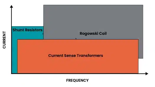
While several sensing technologies are available—including shunt resistors, Rogowski coils, and current sense transformers (CSTs)—the CST stands out when accuracy, galvanic isolation, and efficiency at high frequencies are essential.

Technology landscape: Comparing sensing methods

Selecting the right current sensing technology requires balancing trade-offs in accuracy, cost, power dissipation, isolation, and frequency response.

Technology	Advantages	Limitations	Typical applications
Shunt resistor	Low cost, simple, no phase error	High loss, no isolation	Low-power DC/DC, battery monitoring
Hall-effect sensor	High accuracy, galvanic isolation, DC & AC sensing	Expensive, requires power, temperature sensitive	Industrial drives, medical, precision systems
Current sense transformer (CST)	Accurate, low-loss, isolated, good EMI immunity	No DC response, core saturation at very low frequency	SMPS, AC line monitoring, solar/UPS
Rogowski coil	Wide bandwidth, no core saturation, high current	Needs integrator, poor low-frequency response	Transient analysis, arc fault detection, power quality

Every CST has a minimum usable frequency below which phase shift and amplitude error become unacceptable for control purposes. As frequency decreases, the induced secondary voltage becomes small relative to magnetizing current and burden resistor effects, which leads to increasing phase lag and distortion; true DC components are not transferred but still bias the core flux and can cause flux walking toward saturation if not reset.​

The decision often comes down to whether the application requires high efficiency and strong isolation at high frequency—an area where CSTs consistently outperform alternatives.

Application domains

CSTs are widely adopted wherever high‑frequency AC current must be monitored efficiently and safely.

Typical domains include:

• SMPS and DC‑DC converters: precise peak or average current feedback for regulation, over‑current protection, and current‑mode control.
• High‑voltage monitoring: isolated current measurement in systems requiring basic, functional, or reinforced insulation.​
• Solar inverters and UPS: high‑frequency current feedback in noisy environments, often at elevated bus voltages.​
• Industrial automation and motor drives: robust sensing in EMI‑rich systems, often combined with digital control.
• Automotive and EV battery management: isolated measurement of converter and charger currents, with stringent size and safety constraints.

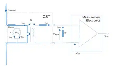
Operating Principles of Current Sense Transformers

The operation of a current sense transformer is grounded in the fundamentals of electromagnetic induction. When an AC current flows through the primary winding, it induces a proportional current in the secondary. This secondary current, when passed through a terminating resistor, produces a measurable voltage directly proportional to the original current.

Ideal relationships

(1) Sense current vs. primary current (ideal CST)

$I_{\text{Prim}} = N \cdot{I_{\text{sense}} }$

Where N means a turn-ratio. Voltage sense is a direct measurement of a primary current I_prim

(2) Sense voltage across terminating resistor

$V_{\text{sense}} = R_T \cdot \frac{I_{\text{prim}}}{N}$

Non-ideal behavior and losses

Flowing primary current slightly differs from measured current value, as the core of current sense transformers needs to be magnetized by magnetizing current. Hysteresis losses (I_Fe) are typically negligible for CSTs. The magnetizing current can be identified from basic parameters as a source of amplitude error.

(3) Primary current composition

Magnetic modeling and optimization

To optimize CST parameters, magnetic Finite Element Method (FEM) analysis is used. Magnetic field distribution analysis helps determine magnetic losses and phenomena related to phase shift between measured and sensed current values.

Comparator-based measurement

A CST integrates easily into analog or digital measurement systems. The sense voltage—i.e., the voltage drop across the external terminating resistor R_T – is commonly used as the comparator input voltage.

(4) Comparator input and output behavior

Comparator’s tasks is to compare measured V_sense value to assigned reference voltage V_ref, where V_ref value typically defines maximum voltage drop we can measure on R_T – under I_sense is flowing:

As result – we get final referenced output voltage V_out, which can be directly used for discrete or analog regulation systems or for monitoring purpose.

Current sense transformer selection guidelines

Accurate and reliable CST implementation depends on proper selection of both the magnetic component and the measurement network.​

Key design parameters include:

• RMS current rating to avoid copper and core overheating under maximum load.​
• Volt‑second product and core flux density to ensure adequate margin to saturation over the full duty‑cycle and frequency range.​
• Terminating resistor $R_T$, which defines sense voltage level, sensitivity, and bandwidth.​
• Isolation voltage and insulation system (basic, functional, reinforced) to satisfy safety standards and creepage/clearance requirements.​
• Mechanical constraints (package, pad layout, window size) and primary conductor style (PCB trace, wire, busbar).​

A practical design flow can be split into three main steps.

Step 1. Product series choice based on safety

The first step is to define application constraints: maximum current, insulation level, operating voltage, and form‑factor limits.​

YAGEO catalog CSTs, for example, offer solutions up to about 1.5 kV with appropriate creepage and clearance for reinforced insulation, and package families optimized for continuous currents up to tens of amperes and switching frequencies into the low‑MHz range. Full‑custom CSTs are often used when current exceeds catalog ranges or when non‑standard busbar or PCB geometries are required.

The catalog portfolio covers mechanically optimized constructions for applications up to 50 A with a wide range of turns ratios. Some products support measurement frequencies up to 2 MHz. Full custom designs are available for wider current ranges.

Step 2 – Part Number Choice, Working Point, and Terminating Resistor

With a suitable series identified, the next step is to select the turns ratio and calculate the operating flux density and burden resistor.​

Input Parameters. Typical inputs are:

• Peak primary current $I_{\text{pk}}$
• Switching frequency $f$ and duty cycle $D$
• Comparator reference voltage $V_{\text{ref}}$ (which sets $V_{\text{sense,max}}$)
• Effective core area $A_e$ (from datasheet)

Working point and flux density

Selection starts with CST turns ratio based on working point (flux density B) under given conditions: frequency (f), duty cycle (D), and V_ref. Datasheets specify the effective core area A_e used in flux estimations.

(5) Flux density working point (conceptual)

To stay in the linear part of the core B/H characteristic, the working point B should typically be within 250–2200 Gauss, with the absolute maximum specified in the datasheet. This region determines a feasible solution domain for part selection.

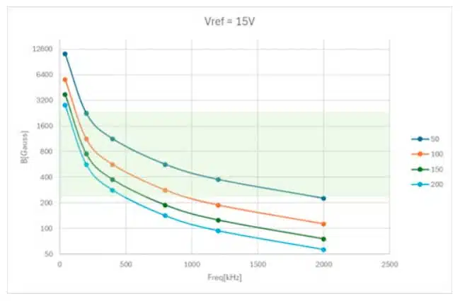
Higher frequencies generally require lower turns counts and higher V_ref, while lower frequencies require higher turns ratios and may use lower V_ref. The turns ratio N impacts sensitivity: higher N lowers the working point and V_sense, reducing sensitivity.

Terminating resistor calculation

Once a part number is selected, determine the terminating resistor value.

(6) Terminating resistor from peak conditions

Step 3. Measurement error, signal delay & sensitivity

Analyze amplitude and phase shift error. Amplitude error is mostly caused by CST losses, where magnetizing current plays a significant role and is typically small and linear (often < 2%). Phase error depends on burden and parasitics and should be minimized during design.

(7) Amplitude error due to magnetizing current

(8a) Phase shift (general)

(8b) Phase shift (simplified when R_T ≫ R_DC,sec)

(8c) Maximum phase error estimate

Sensitivity

(9a) Sensitivity (V/A)

(9b) Sensitivity error

Case study: High-accuracy CST performance

Consider an automotive current sensing application such as battery management or DC‑DC converter current monitoring, with the following conditions:​

• Reference voltage $V_{\text{ref}}=15\text{V}$
• Estimated peak primary current $I_{\text{pk}}=29\text{A}$
• Frequency $f=200\text{kHz}$
• Duty cycle $D=0.8$
• Mechanical maximum size around 13 mm × 11 mm × 8 mm

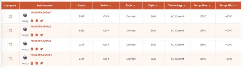
A catalog series (for example, YAGEO CSFA family) is selected that meets insulation and size constraints. Within the PMS9494 range, turns ratios of 1:50, 1:100, 1:150, and 1:200 are available; flux‑density calculations show that 1:50 slightly exceeds the recommended 2200 Gauss limit, while 1:100 falls nicely in the mid‑range, leaving margin for variations in frequency, current, and duty cycle.​

Using $N=100$, the burden resistor required at 29 A peak and 15 V reference is approximately:

$R_T={\displaystyle \frac{15\cdot 100}{29}}\approx 52\mathrm{\Omega }$

A standard 50 Ω value is a convenient practical choice and keeps the secondary DCR contribution negligible.​

Magnetizing current under these conditions is on the order of a fraction of a milliampere, resulting in amplitude error well below 0.01%. Simplified phase‑shift calculations yield roughly 1 degree of phase angle at 200 kHz, corresponding to a phase‑related amplitude error of about 0.0164%, demonstrating the extremely high accuracy achievable with a correctly selected CST.​

The resulting sensitivity is:

$\text{sensitivity}\approx {\displaystyle \frac{14.5\text{V}}{29\text{A}}}\approx 0.5\text{V/A}$

showing how burden choice directly sets volts‑per‑ampere gain and influences effective dynamic range at the comparator or ADC input.

Designing a Custom Current Sense Transformer

When catalog parts cannot meet the mechanical or current requirements, custom CSTs can be designed around the same principles.​

Core Choice – Key considerations include:

• Ferrite material tailored to the frequency range and acceptable flux density, with targets for $B_{\text{max}}$ that keep hysteresis and core loss under control.​
• Trade‑off between higher $B_{\text{max}}$ (for compact designs) and phase error/saturation margin over the full load and temperature range.​

Window Utilization – The physical window must accommodate the chosen primary conductor style, secondary winding, insulation layers, and creepage/clearance:​

• Busbar, PCB copper, or wire primaries set different constraints on minimum window height and insulation thickness.
• Fill factor guidelines ensure manufacturability and robust insulation, while leakage inductance is kept under control to preserve bandwidth.​

Loss and Temperature – A quick loss and temperature‑rise estimation combines:

• Copper loss in primary and secondary windings from RMS currents and DCR.​
• Core loss from AC flux density and operating frequency, using material loss curves or Steinmetz‑type equations.​

These calculations define whether the selected core and winding scheme meet thermal limits across the intended ambient range.

Step 1: Series choice

Automotive applications require functional insulation. With the noted mechanical constraints, select CSFA series and use the YAGEO Group product selector to locate a suitable range.

Step 2: Part selection and working point

Open the datasheet to review parameters. In this case, four turns ratios are available for the PMS9494 product range.

To better understand, we calculate working point based (flux density B) according to Eq.5 based on our automotive application conditions: Freq. = 200kHz, Vref=15V, DutyCycle=0.8. This equation is also specified in datasheet (Fig. 10, Notes, Pkt 4). Calculations can be systemized as in Table 2:

N	DutyCycle	Vref [V]	Freq [kHz]	Ipk [A]	B [Gauss]	Rsense [Ω]
50	0.8	15	200	29	2256	25.86207
100	0.8	15	200	29	1128	57.72414
150	0.8	15	200	29	752	77.58621
200	0.8	15	200	29	564	103.483

The N=50 option exceeds the suggested limit of B = 2200 Gauss and is excluded. The 1:100 option (PMS9494.100NLT) places B mid-range within the recommended window, providing flexibility for wider switching frequency or overcurrent.

From Eq. (6), the terminating resistor for the selected part is approximately R_T ≈ 50 Ω. The secondary winding DCR is < 10% of R_T and has negligible influence on phase shift under these conditions.

Error and sensitivity estimates

Previous calculated values of B and RT allows us to calculate the amplitude error of the magnetizing current:

Amplitude error due to magnetizing current is very small. Example calculation yields approximately 0.00154%, indicating the magnetizing current component is not measured.

Simplified phase shift calculation indicates a very low signal shift

In this configuration, the measurement error is only 0.0164% and demonstrates exceptional accuracy achievable with well-designed CSTs.

Sensitivity of selected part number under application requirements will be:

Choice of terminating resistance influence sensitivity and sensitivity error.

Behavior Under Fault and Overload Conditions

Under overload or short‑circuit conditions, both peak flux density in the core and power dissipation in the burden resistor increase significantly.

Important checks include:

• Estimating peak flux during worst‑case pulses to ensure saturation is either avoided or its impact on protection accuracy is acceptable.
• Ensuring the burden resistor rating (and any clamping components) can withstand transient energy without failing.
• Verifying creepage and clearance distances and insulation design under surge and fault voltages, especially in high‑voltage systems.​

Protection schemes often add diodes and clamps to manage reset and overvoltage, as discussed in the SMPS application section below.

PCB Layout and EMC Considerations

Good PCB practice is crucial to preserve CST accuracy and minimize EMI issues.​

Key layout rules:

• Minimize loop area between primary return path and secondary/burden loop to reduce susceptibility to common‑mode noise and radiated fields.​
• Keep secondary leads and the burden resistor physically close, use short traces, and apply Kelvin connections where precision is required.​
• Treat the sense circuitry as a small‑signal network; separate its ground references from high‑dv/dt nodes using star‑point grounding and, where appropriate, split planes or local filtering.

These layout practices are particularly important in SMPS designs, where CST signals interface directly with high‑speed current‑mode controllers.

Application in Switched‑Mode Power Supplies

Current sense transformers are widely used in SMPS controllers to monitor peak or average inductor current with high efficiency and isolation. Here is a practical framework example for deploying CSTs in this role.

Basic SMPS Use Case

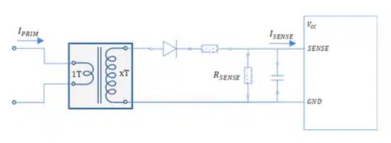
In a typical implementation, a 1‑turn primary is formed by the power trace or lead that carries the converter’s inductor or switch current. The CST secondary, with many turns, drives a burden resistor that develops a low‑voltage signal proportional to primary current, which is then fed into a controller’s current sense input.

The basic relationship:

$V_{\text{out}} = \dfrac{I_{\text{pri}} \cdot R_T}{N_{\text{sec}}}$

shows that, for a given primary current, the designer chooses $R_T$ and $N_{\text{sec}}$ to achieve the desired maximum sense voltage (for example, 1 V/A scaling).

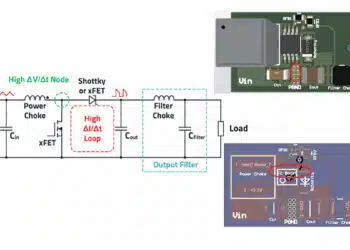
Core Reset and Diode Usage

For high duty‑cycle operation, a key design requirement is ensuring that the CST core is reset each switching period to prevent flux walk and saturation.

A common practice is to place a diode in series with the secondary, across the burden network, so that during the off‑time the core sees a reverse voltage and returns to zero flux, while the reset voltage is isolated from the controller input. A Zener diode may also be added to clamp the secondary voltage during fault conditions and protect both the CST and downstream circuitry.

Without proper reset, residual flux accumulates each cycle, causing the sensed current to appear lower than the true primary current and potentially driving the controller into destructive over‑current conditions.

Turns Ratio Trade‑Offs

Off‑the‑shelf CST families often offer multiple turns ratios in the same package size. Design trade‑offs when choosing a higher versus lower turns ratio include:

• Higher turns ratio improves signal‑to‑noise ratio by producing a larger secondary current and thus higher voltage across a given $R_T$, but increases winding resistance and leakage inductance.
• Higher turns ratio generally reduces flux density for a given output voltage, which helps avoid saturation and reduce core loss, but may slightly shrink bandwidth due to higher impedance.
• Lower turns ratio supports higher primary current (for the same core size) and can improve bandwidth, but may require lower $R_T$ and reduce signal amplitude.

Analysis shows that, for a given package, different turns ratios can be optimized to balance efficiency, accuracy, and bandwidth, and that online selection tools can automate flux‑density checking to avoid saturation.

SMPS Application Examples

Example 1 – LTC3706 Secondary‑Side Synchronous Forward Controller

Analog Devices’ LTC3706 controller documentation compares CST‑based sensing with resistive methods for high‑efficiency, high‑output‑voltage converters.

In one example, a current sense transformer on the secondary side monitors inductor current in a synchronous forward topology. The CST provides:

• Isolation between control and power domains.
• Lower power loss versus shunt sensing at high current.
• High usable frequency range, well aligned with the controller’s switching frequency and control bandwidth.

The CST sense voltage is fed into the controller’s current sense pin, and the turns ratio plus burden are chosen so that the maximum expected current corresponds to the controller’s internal sensing threshold.

Example 2 – TI TIDM‑02009 EV Traction DC‑DC Converter

Texas Instruments’ TIDM‑02009 ASIL‑D‑assessed traction DC‑DC converter reference design uses two Coilcraft CST2010‑100L 1:100 CSTs to sense primary inductance current in a bidirectional converter linking a 400/600 V bus to a 12 V battery.

The converter employs peak current‑mode control, with the CSTs providing isolated feedback of high‑speed current waveforms. The CSTs are selected to:

• Support the full operating current range without core saturation.
• Deliver sufficient sense voltage at the controller input for robust noise immunity.
• Meet automotive isolation and reliability requirements.

This example illustrates how catalog CSTs can be integrated into safety‑critical EV systems using standard design flows and online selection tools.

Integrated Design Considerations

Bringing together the calculation and application perspectives, a practical CST design and selection process for SMPS and automotive systems involves:

1. Defining electrical, safety, and mechanical requirements (current range, bus voltage, insulation class, ambient and size).
2. Choosing a CST series and tentative turns ratio that satisfy insulation and size constraints while keeping flux density within the recommended window.
3. Calculating the burden resistor to map peak current to the desired sense voltage, checking resistor power and controller input limits.
4. Estimating amplitude and phase errors from magnetizing current and parasitic elements, verifying that they are acceptable over the entire operating frequency range.
5. Implementing appropriate core reset and secondary protection (diodes, clamps) to prevent flux walk and overvoltage during faults.
6. Validating performance in circuit through measurements or simulation, and iterating turns ratio or burden value if necessary.

By following this structured flow, designers can confidently exploit the advantages of current sense transformers in high‑performance power converters while avoiding common pitfalls related to saturation, bandwidth, and noise.

Conclusion

Current sense transformers combine high accuracy, galvanic isolation, and low loss, making them a technology of choice for high‑frequency AC current measurement in SMPS, solar inverters, UPS, industrial automation, and automotive systems. With a disciplined selection and calculation process, errors well below 1% in both amplitude and phase are achievable, even in compact, high‑current applications.

As energy efficiency accelerates, CSTs will continue enabling next-generation power systems. CSTs exhibit low measurement error compared to shunts and Rogowski coils due to minimal temperature rise, shielding against external EM fields, and lower energy dissipation than shunts.

FAQ about Current Sense Transformers