

Fringing field effects at air gaps represent a significant but often underestimated source of additional winding losses in magnetic components.
Jonas Mühlethaler, CTO at Frenetic, presented a detailed methodology for accurately modeling air-gap reluctance, calculating the resulting magnetic field distribution, and predicting proximity losses in inductors and transformers.
The fringing field challenge
When magnetic flux passes through an air gap in a magnetic core, it does not travel in perfectly straight lines. Instead, the flux fringes outward near the gap edges, penetrating into the winding window where conductors are located. This perpendicular magnetic field induces eddy currents in the windings, creating additional magnetic losses beyond simple DC resistance—an effect known as proximity loss.
Traditional design approaches often use simplified approximations, such as assuming a homogeneous field distribution or empirically increasing the effective air-gap cross-sectional area. However, these methods can lead to significant errors in loss estimation and saturation current prediction, particularly for complex air-gap geometries.
Three-step modeling methodology
Step 1: Accurate air-gap reluctance calculation
The foundation of fringing field analysis is an accurate reluctance model. Rather than treating the magnetic circuit as a simple resistor network, the methodology employs a building-block approach based on the Schwarz-Christoffel transformation.
This mathematical technique allows any air-gap geometry to be decomposed into fundamental puzzle-piece elements. For each element, the reluctance can be calculated by transforming the complex geometry into an equivalent parallel-plate capacitor configuration where the field is homogeneous. The reluctances of individual building blocks are then combined in series and parallel to represent the complete air gap.
Because real air gaps are three-dimensional, the model calculates fringing factors in two orthogonal planes (y-z and x-z) and multiplies them to obtain a 3D correction factor σ. The actual air-gap reluctance is then:
where is the air‑gap reluctance, is the physical gap length, is the permeability of free space, is the geometric cross‑section of the gap, and is a dimensionless fringing factor that accounts for flux spreading in three dimensions. The fringing factor effectively increases the cross-sectional area to account for flux spreading.
Validation against finite-element method (FEM) simulations demonstrated that this approach matches FEM results accurately across a wide range of air-gap dimensions, while simplified methods can overestimate reluctance by orders of magnitude (note the logarithmic scale in the validation plots). Inductance measurements on an E55/28/21 core with 80 turns confirmed that the new approach predicts measured values far more closely than models neglecting fringing.
Step 2: Determining the magnetic fringing field
Once the accurate reluctance is known, the next challenge is to calculate the magnetic field distribution in the winding window. The key insight is to replace each air gap with a fictitious point current whose magnitude equals the magnetomotive force (MMF) drop across the gap:
where MMF is the magnetomotive force drop across the gap and is the magnetic flux through the gap. This MMF is modeled as an equivalent fictitious current source when computing the fringing field distribution. This MMF value determines the equivalent current that produces the same field pattern as the physical air gap.
With the air gaps represented as currents and the core material treated as infinitely permeable, the method of images (or mirroring method) is applied. Physical boundaries are replaced by mirror images of all conductors (real windings plus fictitious air-gap currents), creating a planar array of current sources. The magnetic field at any point in the winding window is then calculated using Ampère’s law and superposition, summing contributions from all current sources.
This mirroring is performed separately for inner winding windows (surrounded by core material on all sides) and outer winding windows (e.g., around the center leg of an E-core, where material exists only on one side).
Step 3: Calculating winding losses
With the magnetic field distribution known, proximity losses in the conductors can be calculated. For solid round wire, the losses depend on the external magnetic field penetrating the wire and are expressed using Kelvin functions:
for solid round wire, where is the proximity‑loss power in the conductor, is the DC resistance, is the external magnetic field amplitude at the conductor location, and is a dimensionless function of a normalized frequency parameter (based on Kelvin functions) that captures skin and proximity effects. is a frequency- and diameter-dependent factor and is the calculated external field.
For litz wire, the model accounts for both the external field and an internal proximity effect caused by mutual coupling between strands. The internal field is approximated assuming homogeneous current distribution across the bundle:
for litz wire, where is the number of strands, , is the DC resistance of a single strand, is the internal field caused by mutual coupling between strands (approximated assuming homogeneous current distribution), and is the corresponding dimensionless Kelvin‑function term for the strand diameter and operating frequency.
An important simplification is that the model neglects the magnetic field generated by the induced eddy currents themselves. This assumption remains valid provided the design stays below a maximum frequency threshold that depends on wire diameter and permeability. Validation showed errors below 5% for well-designed magnetics below this frequency, and below 25% even above it. For high-frequency designs requiring operation above this limit, switching to litz wire with smaller strand diameters raises the threshold and maintains accuracy.
Practical implications for design engineers
Improved saturation current prediction
Accurate reluctance modeling is critical for predicting saturation behavior. In one test case, neglecting fringing field effects led to a calculated saturation current of 4.6 A, while the measured value was only 3.7 A. The new approach predicted 3.6 A, closely matching the measurement. Overestimating saturation current by 25% could lead to core saturation in the field, causing catastrophic performance degradation or failure.
Optimization of winding placement
Understanding the spatial distribution of fringing fields allows designers to position windings strategically. Areas of high fringing field should be avoided where possible, or if unavoidable, litz wire with finer strands can be used to reduce proximity losses.
Parallel winding considerations
A question from the webinar audience highlighted that parallel conductors on the same core can experience uneven current sharing due to circulating currents induced by fringing fields. This can lead to one conductor carrying significantly more current than another, increasing losses and thermal stress. Twisting parallel wires is one mitigation strategy, though modeling this effect requires advanced techniques such as FEM solvers that can track current distribution among parallel paths.
Design-in notes for engineers
- Reluctance model limitations: The approach is mathematically rigorous and has no fundamental theoretical limitations for the geometries tested. Edge cases involving complex flux paths between adjacent core sections can be handled by adding window-fringing reluctances in parallel, though parameterization may require care.
- Frequency validity range: Frequency validity range: The Kelvin‑function approach for proximity loss is valid up to a maximum frequency that depends primarily on conductor diameter and material properties, because above this point the field generated by eddy currents themselves can no longer be neglected. Designs operating above this threshold should use litz wire with smaller strand diameters to extend the valid frequency range.
- Tool implementation: The complexity of the calculations (Schwarz-Christoffel transformations, method of images, Kelvin functions) makes manual calculation impractical. However, once coded into a design tool, these equations execute efficiently and provide accurate results without requiring FEM simulation for every iteration.
- Core geometry applicability: The building-block reluctance model applies to common core types including E-cores, EI-cores, and center-gapped inductors. Any air-gap geometry can be decomposed into fundamental elements and accurately modeled.
Conclusion
Accurately modeling fringing field losses in magnetic components requires a three-stage approach: precise air-gap reluctance calculation using conformal mapping techniques, field distribution analysis using equivalent currents and the method of images, and frequency-dependent proximity loss estimation using analytical or semi-analytical methods.
This methodology, implemented in modern design tools, enables engineers to predict saturation currents within a few percent, optimize winding placement to minimize losses, and avoid the time and cost of full FEM simulation during initial design iterations. For inductors and transformers operating in power electronics applications—including PFC stages, DC-link filters, onboard chargers, and industrial drives—this level of accuracy translates directly into improved efficiency, thermal performance, and reliability.
Source
This article is based on a technical webinar presented by Jonas Mühlethaler, CTO at Frenetic, detailing the theoretical foundations and practical implementation of fringing field loss modeling in magnetic component design. The methodology draws on research conducted during Dr. Mühlethaler’s PhD at ETH Zurich, where he specialized in magnetic design optimization.