AC Line Filter Calculation, Design and LT Spice Simulation

A single-phase AC line filter for a switch-mode power supply can be dimensioned with a handful of equations once the unfiltered interference spectrum is known. This article shows the complete workflow for power-supply and EMC design engineers: pre-compliance measurement, calculation of a single-stage and a two-stage filter, LTspice simulation, EMC-lab verification, the safety calculations for varistor, leakage current and discharge resistor, and the layout and core-material choices that decide whether the calculated insertion loss is reached in practice.

How to Measure Filter Performance: Insertion Loss, VNA Fixtures and CM/DM Separation

Passive Filter Technologies Compared: LC, Ferrite, Feedthrough, Ceramic, Cavity, Microstrip, SAW and BAW

Würth Elektronik Releases Common-Mode Chokes for 100 V Data and Power Lines

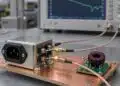
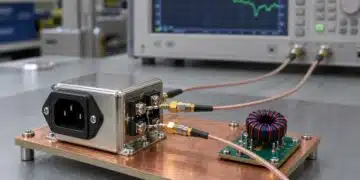
The method follows the Würth Elektronik webinar by Andreas Nadler and the associated application note ANP015 [1], [2]. An isolated 25 W flyback converter switching at 300 kHz serves as the interference source, and a filter board carrying both filter variants is measured against the Class B limits. The underlying LC low-pass principles are covered in basic filter circuits explained.

Key Takeaways

Measure the unfiltered DUT first: the required insertion loss at the switching frequency (here about 40 dB including roughly 10 dB margin) sets every component value; without a measurement, design for at least 40 dB in both CM and DM.
A single-stage LC filter gives 40 dB per decade above its cut-off frequency, a two-stage filter 80 dB per decade, so the two-stage version reaches the same attenuation at 300 kHz with smaller components and is up to about 30 dB better at higher frequencies.
The common-mode inductance follows from the Y-capacitance, which is capped by the permitted leakage current; the differential-mode inductance is the leakage inductance of the common mode choke, read from its DM impedance curve.
Nominal choke inductance is specified at low frequency (often 10 kHz); MnZn and nanocrystalline chokes with the same 1 mH rating differ by a factor of about four in effective inductance at 1 MHz, so design with the impedance at the frequency of interest.
Varistor, Y-capacitor leakage current and X-capacitor discharge resistor must be calculated with worst-case tolerances; for the discharge resistor, use the peak mains voltage, not the RMS value.
Layout decides the high-frequency result: low-inductance PE connection of the Y-capacitors, no copper under the common mode choke, no stub traces and adequate spacing between input and output.

Common Mode and Differential Mode Interference

Conducted interference from a switch-mode power supply travels on two paths. Differential-mode (DM) current flows out on line (L) and back on neutral (N); common-mode (CM) current flows in the same direction on L and N and returns via protective earth (PE), mostly through parasitic capacitances of the switching node and the transformer. A line filter has to attenuate both, and each path uses different filter components.

LISN and separation of CM and DM

An EMC acceptance test always measures the sum of both paths. For filter design it is far more useful to measure CM and DM separately, which requires a LISN (line impedance stabilisation network) whose two measurement outputs L_RF and N_RF can be used simultaneously. The LISN contains two 50 Ω measuring resistors: for DM they appear in series (100 Ω), for CM in parallel (25 Ω) [1]. With both outputs connected to two 50 Ω oscilloscope inputs, the math function of the oscilloscope gives the DM and CM interference voltages, Eq. (1) and Eq. (2):

V_{DM} = \frac{V_{L,RF} – V_{N,RF}}{2} \tag{1}

V_{CM} = \frac{V_{L,RF} + V_{N,RF}}{2} \tag{2}

where V_L,RF and V_N,RF are the voltages at the line and neutral measurement outputs of the LISN.

Pre-compliance measurement with an oscilloscope

The reference measurement in [1] uses a 500 MHz oscilloscope with EMI-debug software and an FFT display in dBµV, a CISPR 16 LISN, a coupling plate and an isolating transformer. Two set-up details matter. First, the vertical scale of each channel should be set just above the measured peak-to-peak level (for example 100 mV full scale for an 85 mV signal) so that the resolution is maximised without overdriving the input. Second, the DUT should run at maximum output load, where the interference level is usually highest.

Without a filter, the flyback converter produces 84 dBµV in both CM and DM at the 300 kHz switching frequency, against a Class B average limit of about 50 dBµV at that frequency. This gives a minimum requirement of 34 dB CM and 27 dB DM insertion loss; the combined CM plus DM spectrum (86 dBµV) needs more than 36 dB [1]. The Class B limits for AC mains ports decrease linearly with the logarithm of frequency from 66 dBµV to 56 dBµV quasi-peak and from 56 dBµV to 46 dBµV average between 150 kHz and 500 kHz [4], which places the average limit at 300 kHz at 50 dBµV and the quasi-peak limit at about 60 dBµV. The average limit is therefore the binding one for this design.

If only a standard LISN without simultaneous outputs is available, the combined spectrum is used as the basis. If no pre-compliance measurement is possible at all, the filter should be designed for at least 40 dB CM and DM insertion loss at the switching frequency [1].

Switching frequencies below 150 kHz

Conducted-emission limits under CISPR 32 Edition 2 start at 150 kHz. If the switching frequency lies below that range, the first harmonic inside the measured spectrum becomes the design frequency: a 70 kHz converter is designed for its third harmonic at 210 kHz [1]. Edition 3 of CISPR 32, circulated as a final draft for voting from October to December 2026, adds Class B emission limits on AC mains below 150 kHz, in line with IEC 61000-6-3:2026 and CISPR PAS 39 [5]. Once adopted and harmonised, converters with low switching frequencies, including PFC stages, will need their fundamental and lower harmonics checked against these limits as well.

Calculation of the Single-Stage Line Filter

A single-stage LC filter is a second-order low-pass with an ideal asymptotic slope of 40 dB per decade above its cut-off frequency. The calculation below treats CM and DM separately, uses ideal components and neglects source and load impedances; the real insertion loss of an AC line filter depends on both, which is why the result is checked by simulation and measurement afterwards.

Cut-off frequency

The attenuation A_fsw obtained at the switching frequency f_SW for a cut-off frequency f_CO is given by Eq. (3); solving for f_CO gives Eq. (4):

A_{fsw} = 40\,\mathrm{dB} \cdot \log_{10}\left(\frac{f_{SW}}{f_{CO}}\right) \tag{3}

f_{CO} = \frac{f_{SW}}{10^{A_{fsw}/40\,\mathrm{dB}}} \tag{4}

With the required 40 dB at 300 kHz, Eq. (5) gives the target cut-off frequency:

f_{CO} = \frac{300\,\mathrm{kHz}}{10^{40/40}} = 30\,\mathrm{kHz} \tag{5}

Y-capacitors and common-mode inductance

The Y-capacitors are chosen first, because the permitted leakage current to PE limits their value in most AC applications (see the leakage-current section below). The single-stage example uses two 4.7 nF Y2 ceramic capacitors; in the CM equivalent circuit they act in parallel, Eq. (6). Background on capacitor safety classes is given in safety capacitors in power electronics; X and Y subclasses and their test regime are defined in IEC 60384-14 [7].

C_{YG} = 2 \cdot C_{Y} = 2 \cdot 4.7\,\mathrm{nF} = 9.4\,\mathrm{nF} \tag{6}

The required common-mode inductance L_CM of the common mode choke follows from the LC resonance condition, Eq. (7):

L_{CM} = \frac{1}{(2\pi f_{CO})^{2} \cdot C_{YG}} = \frac{1}{(2\pi \cdot 30\,\mathrm{kHz})^{2} \cdot 9.4\,\mathrm{nF}} = 3.0\,\mathrm{mH} \tag{7}

3 mH is not a standard value, and common mode chokes have wide inductance tolerances, so a 3.3 mH choke is selected. The cut-off frequency moves to 28.6 kHz and the calculated CM insertion loss at 300 kHz rises to 41 dB [1].

Leakage inductance and X-capacitor

In the DM path the leakage inductance of the common mode choke acts as the series inductor. If the datasheet does not specify it, it can be derived from the DM impedance curve, read in the linear, rising (inductive) region. For the 3.3 mH choke the DM impedance at 1 MHz is 92 Ω, Eq. (8):

L_{DM} = \frac{X_{L}}{2\pi f_{DM}} = \frac{92\,\Omega}{2\pi \cdot 1\,\mathrm{MHz}} = 14.6\,\mathrm{\mu H} \tag{8}

where X_L is the DM reactance read at the frequency f_DM. The X-capacitance then follows from Eq. (9):

C_{X} = \frac{1}{(2\pi f_{CO})^{2} \cdot L_{DM}} = \frac{1}{(2\pi \cdot 30\,\mathrm{kHz})^{2} \cdot 14.6\,\mathrm{\mu H}} = 1.93\,\mathrm{\mu F} \tag{9}

The next standard value, a 2.2 µF / 310 V X2 film capacitor, gives a calculated DM insertion loss of 41 dB. X-capacitors can lose capacitance over their lifetime under poor mains quality and repeated surges, so a margin above the calculated value is advisable [1].

Component placement

The CM interference source of a switch-mode supply has a high impedance, the DM source a comparatively low impedance. For maximum insertion loss the Y-capacitors are therefore placed in parallel with the DUT side and the X-capacitors in parallel with the LISN (mains) side, with the choke between them [3].

Calculation of the Two-Stage Line Filter

A two-stage filter cascades two LC sections. Compared with a single stage it offers four advantages: smaller individual components, better parasitic behaviour (in particular higher self-resonant frequencies of the smaller parts), more design flexibility and an ideal slope of 80 dB per decade instead of 40 dB per decade [1].

Effective cut-off frequency

Eq. (3) and Eq. (4) become Eq. (10) and Eq. (11) with the steeper slope:

A_{fsw} = 80\,\mathrm{dB} \cdot \log_{10}\left(\frac{f_{SW}}{f_{CO}}\right) \tag{10}

f_{CO} = \frac{f_{SW}}{10^{A_{fsw}/80\,\mathrm{dB}}} \tag{11}

For 40 dB at 300 kHz, Eq. (12) gives an effective cut-off frequency of 95 kHz, more than three times higher than for the single stage:

f_{CO} = \frac{300\,\mathrm{kHz}}{10^{40/80}} = 95\,\mathrm{kHz} \tag{12}

A ladder of two identical LC sections has two resonances. Their frequencies f_CO1 and f_CO2 lie at 0.618 and 1.618 times the single-section resonance frequency, which the application note rounds to Eq. (13) and Eq. (14) [1]:

f_{CO1} \approx 0.6 \cdot f_{CO} = 0.6 \cdot 95\,\mathrm{kHz} = 57\,\mathrm{kHz} \tag{13}

f_{CO2} \approx 1.6 \cdot f_{CO} = 1.6 \cdot 95\,\mathrm{kHz} = 152\,\mathrm{kHz} \tag{14}

For the simplified 80 dB per decade analysis to hold, the switching frequency should lie well above f_CO2, so that the resonance overshoot no longer matters. In general the two cut-off frequencies should be at least one octave (2 : 1) apart to avoid overlapping resonance peaks; with identical stages their ratio is 2.6, so the condition is met automatically.

Component values

Two 2.2 nF Y2 capacitors per stage give Eq. (15), and the common-mode inductance per stage follows from Eq. (16):

C_{YG} = 2 \cdot C_{Y} = 2 \cdot 2.2\,\mathrm{nF} = 4.4\,\mathrm{nF} \tag{15}

L_{CM} = \frac{1}{(2\pi \cdot 95\,\mathrm{kHz})^{2} \cdot 4.4\,\mathrm{nF}} = 0.64\,\mathrm{mH} \tag{16}

Allowing for the choke tolerance, a 1 mH choke in a smaller package is selected, which raises the calculated CM insertion loss to 48 dB. Its DM impedance at 1 MHz is 41 Ω, giving Eq. (17) and Eq. (18):

L_{DM} = \frac{41\,\Omega}{2\pi \cdot 1\,\mathrm{MHz}} = 6.5\,\mathrm{\mu H} \tag{17}

C_{X} = \frac{1}{(2\pi \cdot 95\,\mathrm{kHz})^{2} \cdot 6.5\,\mathrm{\mu H}} = 0.43\,\mathrm{\mu F} \tag{18}

A 560 nF / 310 V X2 capacitor per stage is used, for a calculated DM insertion loss of 45 dB [1]. Table 1 compares both designs.

Parameter	Single-stage filter	Two-stage filter (per stage)
Target insertion loss at 300 kHz	40 dB	40 dB
Ideal slope	40 dB/decade	80 dB/decade
Effective cut-off frequency	30 kHz	95 kHz
Y-capacitors	2 × 4.7 nF Y2	2 × 2.2 nF Y2
Calculated / selected L_CM	3.0 mH / 3.3 mH	0.64 mH / 1 mH
L_DM (from DM impedance at 1 MHz)	14.6 µH (92 Ω)	6.5 µH (41 Ω)
Calculated / selected C_X	1.93 µF / 2.2 µF	0.43 µF / 560 nF
Calculated CM / DM insertion loss	41 dB / 41 dB	48 dB / 45 dB
Measured attenuation at 300 kHz (CM + DM)	41 dB	45 dB

Table 1. Single-stage versus two-stage AC line filter for a 25 W, 300 kHz flyback converter; values from [1], recalculated.

Stages with unequal component values

When the two stages use very different values, for example a large inductor L₁ and a small inductor L₂, the transfer function splits into a low-frequency and a high-frequency pole pair, Eq. (19):

\Delta(s) = \left(1 + \frac{s}{\omega_{L} Q_{L}} + \frac{s^{2}}{\omega_{L}^{2}}\right) \cdot \left(1 + \frac{s}{\omega_{H} Q_{H}} + \frac{s^{2}}{\omega_{H}^{2}}\right) \tag{19}

where ω_L and ω_H are the angular frequencies and Q_L and Q_H the quality factors of the two pole pairs. The low pole is set by the larger inductor and the parallel capacitance C_P, the high pole by the smaller inductor and the series capacitance C_S, Eq. (20) and Eq. (21) [1]:

f_{CL} = \frac{1}{2\pi\sqrt{L_{1} C_{P}}}, \qquad C_{P} = C_{1} + C_{2} \tag{20}

f_{CH} = \frac{1}{2\pi\sqrt{L_{2} C_{S}}}, \qquad C_{S} = \frac{C_{1} C_{2}}{C_{1} + C_{2}} \tag{21}

LTspice Simulation of Both Filters

Before a filter goes into schematic and layout, its frequency response should be checked in a circuit simulator. LTspice includes manufacturer models of the chokes and capacitors with their parasitic elements, which makes the simulation far more realistic than the ideal calculation [1], [3].

Simulation set-up

Separate CM and DM test circuits, each terminated with the corresponding LISN impedance.
DM source as a low-impedance voltage source, CM source as a high-impedance current source [3].
Component models with realistic parasitics (ESR, ESL, winding capacitance, core losses).
Elements neglected in the hand calculation included: the Y-capacitors appear in series between L and N in the DM circuit, and the 420 pF parasitic capacitance of the varistor is added to the DM model [1].

Simulation results

Both filters reach 40 dB to 43 dB CM insertion loss at 300 kHz, matching the calculation. From about 350 kHz upwards, the two-stage filter attenuates up to 30 dB more than the single-stage filter, and the same advantage appears in DM [1]. The simulation also shows the self-resonances of the real components, which set the upper limit of useful attenuation for the single-stage design.

Verification in the EMC Laboratory

Conducted emissions from 150 kHz to 30 MHz and radiated emissions from 30 MHz to 1 GHz were measured with the flyback converter, the filter board and an electronic load [1].

Without filter: 84 dBµV at 300 kHz, almost identical to the oscilloscope pre-compliance result.
Single-stage filter: 43 dBµV at 300 kHz, corresponding to 41 dB attenuation, but less than 10 dB margin to the average limit at 21 MHz.
Two-stage filter: 39 dBµV at 300 kHz, corresponding to 45 dB attenuation, and up to 30 dB lower levels than the single-stage filter in the upper conducted range.
Radiated emission: the two-stage filter lowers the field strength by up to 10 dBµV/m above 150 MHz.

Calculation, simulation and measurement agree closely at the switching frequency. Typical causes of deviation at other frequencies are cable inductance, model inaccuracies, component tolerances, saturation of the common mode choke by excessive CM current, parasitic PCB inductance and direct near-field coupling into the filter components [1].

Dimensioning the Varistor between L and N

A metal-oxide varistor between L and N protects the rectifier and the downstream circuit against surges. The design below assumes the worst case for the varistor, a surge generator with 2 Ω output impedance according to IEC 61000-4-5 [6], which drives the highest current. General application rules are summarised in safe use of varistors and common mode chokes in mains filters.

Pulse energy and equivalent pulse duration

The energy absorbed by the varistor is approximated conservatively by an energy-equivalent rectangular pulse built from the peak current and peak voltage of the varistor (marked with a hat) and the equivalent duration t_eq, Eq. (22):

W_{V} = \int_{0}^{T} I_{V}(t) \cdot V_{V}(t)\,dt \approx \hat{I}_{V} \cdot \hat{V}_{V} \cdot t_{eq} \tag{22}

For the 8/20 µs short-circuit current wave, the linear rise (T₁ = 8 µs) and the exponential decay to half value (T₂ = 20 µs) give Eq. (23):

t_{eq} = 0.5 \cdot T_{1} + 1.43 \cdot (T_{2} – T_{1}) = 4\,\mathrm{\mu s} + 17.16\,\mathrm{\mu s} = 21.16\,\mathrm{\mu s} \tag{23}

Worked example

The example in [1] assumes an industrial application whose circuit withstands at most 1 kV (a typical bridge-rectifier value), a 2 kV surge test with 2 Ω generator impedance between L and N, and a 230 V_RMS mains supply. The varistor working voltage must stay above the maximum mains voltage, Eq. (24):

V_{RMS} \gt V_{GRID} \cdot 1.1 = 230\,\mathrm{V} \cdot 1.1 = 253\,\mathrm{V} \tag{24}

A 300 V_RMS type (alternatively 275 V_RMS) with a disc diameter of at least 14 mm is chosen for adequate energy and power rating. Its datasheet clamping voltage of 775 V refers to 50 A, while the surge test drives a much higher current. In the worst case the mains peak voltage (230 V × 1.41 = 325 V) adds to the generator voltage, so the prospective short-circuit current is Eq. (25):

I_{G} = \frac{V_{G} + V_{GRID,pk}}{Z_{G}} = \frac{2\,\mathrm{kV} + 325\,\mathrm{V}}{2\,\Omega} = 1163\,\mathrm{A} \tag{25}

The V/I curve at +10 % tolerance gives a clamping voltage of 1.02 kV at 1163 A. Subtracting it yields a better estimate of the varistor current, Eq. (26), at which the curve gives 971 V, within the 1 kV requirement:

I_{C1} = \frac{V_{G} + V_{GRID,pk} – V_{CLAMP,max}}{Z_{G}} = \frac{2325\,\mathrm{V} – 1020\,\mathrm{V}}{2\,\Omega} = 653\,\mathrm{A} \tag{26}

For the maximum current the curve at −10 % tolerance is used; it gives V_CLAMP,min = 794 V at 653 A, and Eq. (27):

I_{C,max} = \frac{V_{G} + V_{GRID,pk} – V_{CLAMP,min}}{Z_{G}} = \frac{2325\,\mathrm{V} – 794\,\mathrm{V}}{2\,\Omega} = 766\,\mathrm{A} \tag{27}

Pulse life, energy and cooling time

The surge test applies 40 pulses in total. The pulse-life derating curve of the selected varistor allows about 50 pulses at 766 A and 21.16 µs, which is sufficient but leaves limited margin; a 14 mm high-surge type rated for 500 such pulses is the alternative if the specification is stricter [1]. The absorbed energy per pulse is Eq. (28), far below the 140 J rating:

W_{max} = I_{C,max} \cdot V_{CLAMP,min} \cdot t_{eq} = 766\,\mathrm{A} \cdot 794\,\mathrm{V} \cdot 21.16\,\mathrm{\mu s} = 12.9\,\mathrm{J} \tag{28}

With a permissible power dissipation P_DISS of 0.6 W, the varistor needs the cooling time of Eq. (29) between pulses, well inside the 60 s pulse interval of IEC 61000-4-5:

T_{cool} \gt \frac{W_{max}}{P_{DISS}} = \frac{12.9\,\mathrm{J}}{0.6\,\mathrm{W}} = 21.5\,\mathrm{s} \tag{29}

The worst case applies when the positive surge coincides with the 90° and the negative surge with the 270° phase angle of the mains voltage; at other phase angles the varistor load is significantly lower. A real 2 kV surge test on a resistive load measured 700 A peak varistor current and 850 V peak clamping voltage, consistent with the calculation [1]. Three-phase applications with higher working voltages or energies call for larger discs, for example 20 mm.

Leakage Current through Y-Capacitors

Larger Y-capacitors generally lower the CM interference level, but they also increase the leakage current to PE. Depending on the product standard and protection class, permitted values range from a few microamperes in medical equipment to many milliamperes in permanently installed industrial systems; 3.5 mA is a common practical limit for equipment with a protective earth connection [1].

In normal operation N and PE are at almost the same potential. In the fault case with an interrupted connection, the X-capacitors appear in series with one of the Y-capacitors, and the leakage current becomes Eq. (30), with C_XG from Eq. (31):

I_{LEAK} = V_{GRID} \cdot 2\pi f_{GRID} \cdot \left(C_{YL} + \frac{C_{XG} \cdot C_{YN}}{C_{XG} + C_{YN}}\right) \tag{30}

C_{XG} = C_{X1} + C_{X2} \tag{31}

where V_GRID and f_GRID are the mains voltage and frequency, and C_YL and C_YN the Y-capacitors from L and N to PE. For C_X1 = C_X2 = 1 µF, C_Y1 = C_Y2 = 5.6 nF and 230 V / 50 Hz, with +10 % mains voltage and +20 % capacitance tolerance applied to all capacitors (C_XG = 2.4 µF, C_Y = 6.72 nF), Eq. (32) gives:

I_{LEAK} = 253\,\mathrm{V} \cdot 2\pi \cdot 50\,\mathrm{Hz} \cdot \left(6.72\,\mathrm{nF} + \frac{2.4\,\mathrm{\mu F} \cdot 6.72\,\mathrm{nF}}{2.4\,\mathrm{\mu F} + 6.72\,\mathrm{nF}}\right) = 1.07\,\mathrm{mA} \tag{32}

The result is well below 3.5 mA. Because the series X-capacitance is several hundred times larger than C_YN, the leakage current is set almost entirely by the two Y-capacitors, roughly doubling compared with a single Y-capacitor. For applications in which no leakage current is permitted, filters without Y-capacitors are used.

Discharge Resistor for X-Capacitors

Safety standards for plug-connected equipment limit the voltage that remains at the plug pins after disconnection from the mains; ANP015 uses the common design target of less than 60 V within 1 s [1]. The X-capacitors must therefore be discharged through a resistor R_discharge, and the applicable product safety standard defines the exact limit and time.

Total capacitance

The X-capacitors dominate, but a worst-case calculation also includes the parasitic capacitance of the varistor and the two Y-capacitors in series between L and N, Eq. (33), together with +20 % capacitance and +10 % mains tolerance:

C_{tot} = C_{X1} + C_{X2} + C_{MOV} + \frac{C_{YL} \cdot C_{YN}}{C_{YL} + C_{YN}} \tag{33}

Resistor value and power

The capacitor voltage decays exponentially, Eq. (34), which gives the maximum resistance of Eq. (35) and its continuous dissipation of Eq. (36):

V_{discharge} = V_{0} \cdot e^{-t_{discharge} / (R_{discharge} \cdot C_{tot})} \tag{34}

R_{discharge} \lt \frac{t_{discharge}}{C_{tot} \cdot \ln\left(V_{0} / V_{discharge}\right)} \tag{35}

P_{R} = \frac{V_{GRID,RMS}^{2}}{R_{discharge}} \tag{36}

Here V₀ is the capacitor voltage at the moment of disconnection. Because the plug can be pulled at the crest of the mains voltage, the worst case is the peak value, V₀ = 1.1 × 230 V × √2 = 358 V, not the RMS value. For C_tot = 2.1 µF + 20 % = 2.52 µF, t_discharge = 1 s and V_discharge = 60 V, Eq. (37) gives:

R_{discharge} \lt \frac{1\,\mathrm{s}}{2.52\,\mathrm{\mu F} \cdot \ln(358\,\mathrm{V} / 60\,\mathrm{V})} = 222\,\mathrm{k\Omega} \tag{37}

Calculated with the RMS value of 253 V, the same formula would allow 276 kΩ, and a 240 kΩ resistor would need about 1.08 s to discharge from the peak voltage to 60 V. A 200 kΩ resistor, typically built from two or more series resistors, meets the requirement with margin and dissipates Eq. (38) continuously:

P_{R} = \frac{(253\,\mathrm{V})^{2}}{200\,\mathrm{k\Omega}} = 0.32\,\mathrm{W} \tag{38}

Besides power, the resistor chain must meet the required dielectric strength and the creepage and clearance distances between L and N. The continuous dissipation is also a standby-loss contribution, which is relevant for products with tight no-load power requirements.

Line Filter Layout and Component Instructions

Two aspects govern the layout: electrical safety and the parasitic effects that determine high-frequency insertion loss. Creepage and clearance distances depend on working voltage, pollution degree, insulating material and overvoltage category, and only components with the required safety approvals (for example UL or VDE) may be used [1].

Y-capacitor ground: connect the PE reference of the Y-capacitors with the lowest possible inductance, for example through SMT spacer bolts directly to the chassis; a long PE trace destroys their high-frequency effect.
No copper under the choke: filled copper areas beneath the common mode choke increase the input-to-output coupling capacitance and degrade insertion loss at high frequencies.
No stub traces: route conductors directly through the component pads instead of branching to them, to minimise connection inductance.
Spacing: place filter components at a deliberate distance from each other and from interference sources to limit near-field coupling of H and E fields.
Input and output separation: keep the unfiltered input wiring physically away from the filtered output so that interference cannot bypass the filter.

Core Materials for Common Mode Chokes

The common-mode inductance used in the calculation is only valid if it is still present at the design frequency. The core material of the choke decides how far that holds. Common mode chokes for line filters use three main materials; the properties of the nanocrystalline variant are explained in nanocrystalline soft magnetic core materials explained.

Core material	Strongest CM insertion loss	Notes
Manganese-zinc ferrite (MnZn)	About 50 kHz to 5 MHz	High permeability; inductance drops at low temperature and vanishes above the Curie point
Nanocrystalline (NC)	Widest bandwidth	Impedance flattens from about 50 kHz; stable over temperature
Nickel-zinc ferrite (NiZn)	About 5 MHz to 500 MHz	Low permeability; suited to high-frequency suppression

Table 2. Core materials for common mode chokes in AC line filters [1].

Nominal inductance versus impedance at the design frequency

Nominal inductance is often measured at 10 kHz. Two 1 mH chokes in the same package, one MnZn and one nanocrystalline, have almost identical curves at 10 kHz, but the nanocrystalline curve flattens above about 50 kHz and the MnZn curve changes above about 300 kHz. At 1 MHz the MnZn choke shows 3.91 kΩ, equivalent to 0.62 mH, the nanocrystalline choke 0.915 kΩ, equivalent to 0.146 mH [1]. The filter should therefore be designed from the CM impedance at the switching frequency, and the self-resonant frequency of the choke should lie well above it, since impedance and insertion loss fall beyond resonance.

Temperature and saturation

MnZn permeability, and with it the CM inductance, drops markedly at very low temperatures; above the Curie point (180 °C for the measured choke) the core loses its magnetic properties and only the air-coil impedance of the winding remains. Nanocrystalline cores show no such temperature dependence, which together with their broadband impedance makes them the first choice in many applications [1].

Common mode chokes have no air gap, so all core materials saturate sharply with rising CM current. In typical power supplies the CM current is below 10 mA and uncritical. Motor inverters are the main exception: high capacitive coupling to PE lets large CM currents circulate. A choke that runs hotter than its rated current suggests, or a filter that underperforms, may be saturated [1].

Integrated Line Filters as an Alternative

Where a discrete design is not justified, integrated line filters contain all filter components except the varistor in a metal housing. Single- and two-stage versions exist, as do variants without Y-capacitors for zero-leakage applications; the series described in [1] covers 1.5 A to 20 A and is certified to IEC/EN/UL 60939-2. Two installation rules decide their performance: a solid, low-impedance bond between the metal housing and PE or chassis, and input and output cables routed apart from each other.

Design and Selection Checklist

The checklist summarises the decisions and datasheet parameters that determine whether a discrete AC line filter meets its targets.

Requirement: unfiltered CM and DM spectrum at maximum load, required insertion loss at the switching frequency (or first relevant harmonic) plus about 10 dB margin.
Topology: single stage for moderate requirements; two stages for higher attenuation, smaller components and better high-frequency performance.
Y-capacitors: Y1/Y2 subclass per IEC 60384-14, capacitance capped by the leakage-current limit including +20 % tolerance and the fault case.
Common mode choke: CM impedance at the design frequency (not only nominal inductance), DM (leakage) impedance, self-resonant frequency, rated current and temperature rise, core material, saturation under expected CM current.
X-capacitors: X1/X2 subclass, capacitance margin for ageing under surge stress, rated voltage (for example 310 V AC).
Varistor: working voltage at least 1.1 × nominal mains, clamping voltage at the real surge current versus the withstand voltage of the protected parts, pulse-life derating, energy and cooling time.
Discharge resistor: value from the peak mains voltage and worst-case capacitance, power dissipation, voltage rating, creepage and clearance.
Catalogue versus custom: integrated filters save design and approval effort; discrete filters allow optimisation for size, cost and specific spectra.
Verification: LTspice with manufacturer models and realistic source impedances, then pre-compliance and accredited EMC measurements, conducted and radiated.

Conclusion

An AC line filter can be dimensioned with simple mathematics once a reference measurement of the unfiltered converter defines the required insertion loss. The cut-off frequency follows from the filter order, the Y-capacitance from the leakage-current budget, the CM inductance from the resonance condition and the X-capacitance from the leakage inductance of the choke. In the 25 W, 300 kHz flyback example, calculation, LTspice simulation and EMC-lab measurement agree within a few decibels at the switching frequency. The two-stage filter reaches the target with smaller components and performs up to 30 dB better in the higher conducted range and up to 10 dBµV/m better in radiated emission. Choke core material, worst-case safety calculations and a disciplined layout determine whether the calculated values hold over frequency, temperature and lifetime.

FAQ

How much insertion loss does an AC line filter need?

The requirement follows from a reference measurement of the unfiltered device: the difference between the measured level and the applicable limit at the switching frequency, plus a margin of about 10 dB. In the flyback example this gives about 40 dB for both common mode and differential mode. Without a measurement, a design target of at least 40 dB at the switching frequency is a practical starting point.

What is the difference between a single-stage and a two-stage line filter?

A single-stage LC filter attenuates with an ideal slope of 40 dB per decade above its cut-off frequency, a two-stage filter with 80 dB per decade. The two-stage design therefore reaches the same attenuation with a higher cut-off frequency and smaller components, has better self-resonance behaviour and in the measured example performs up to 30 dB better in the higher conducted frequency range.

How do I calculate the common mode choke inductance?

First fix the Y-capacitance, which is limited by the permitted leakage current. The two Y-capacitors act in parallel in the common-mode circuit. The inductance then follows from the resonance condition: one divided by the square of two pi times the cut-off frequency, multiplied by the total Y-capacitance. Choose the next standard value above the result to cover the wide inductance tolerance of common mode chokes.

Where does the differential mode inductance of a line filter come from?

In a typical discrete filter the leakage inductance of the common mode choke provides the differential-mode inductance. If the datasheet does not specify it, read the differential-mode impedance in the linear, rising part of the impedance curve, for example at 1 MHz, and divide it by two pi times that frequency. The X-capacitor is then calculated from this inductance and the cut-off frequency.

Why can two common mode chokes with the same inductance filter differently?

Nominal inductance is usually measured at 10 kHz, but permeability depends on frequency, temperature and current. In the example, a 1 mH manganese-zinc choke still provides about 0.62 mH at 1 MHz, a 1 mH nanocrystalline choke only about 0.15 mH. Designing from the common-mode impedance at the switching frequency avoids this error. Saturation by excessive common-mode current also reduces inductance.

How is the leakage current of Y-capacitors calculated?

The leakage current equals the mains voltage times two pi times the mains frequency times the effective capacitance to protective earth. In the fault case the X-capacitors are in series with one Y-capacitor, so both Y-capacitors contribute. Use worst-case tolerances, for example plus 10 percent mains voltage and plus 20 percent capacitance, and compare the result with the limit of the applicable standard, often 3.5 mA.

How do I size the discharge resistor for X-capacitors?

The resistor must discharge the total capacitance between the lines, including X-capacitors, varistor capacitance and the series Y-capacitors, below the permitted voltage within the required time, for example 60 V within 1 s. Use the peak mains voltage with tolerance as the starting voltage and plus 20 percent capacitance. Then check power dissipation, voltage rating, creepage and clearance of the resistor chain.

How to Design a Single-Phase AC Line Filter

Step-by-step procedure for dimensioning and verifying a discrete single-phase AC line filter for a switch-mode power supply.

Measure the unfiltered spectrum
Connect the device at maximum load to a LISN, record the common-mode and differential-mode interference spectra and determine the excess over the limit at the switching frequency or the first harmonic above 150 kHz.
Define the required insertion loss
Add a margin of about 10 dB to the measured excess. Without a measurement, use at least 40 dB at the switching frequency for both common mode and differential mode.
Choose the filter order and cut-off frequency
Calculate the cut-off frequency from the required attenuation with 40 dB per decade for a single-stage or 80 dB per decade for a two-stage filter.
Select the Y-capacitors and the common mode choke
Fix the Y-capacitance from the leakage-current budget, calculate the common-mode inductance from the resonance condition and select the next standard value, checking the choke impedance at the design frequency.
Calculate the X-capacitor
Derive the leakage inductance from the differential-mode impedance curve of the choke and calculate the X-capacitance for the same cut-off frequency, adding margin for capacitance loss over lifetime.
Add the protection and safety parts
Dimension the varistor for the surge test, check the leakage current with worst-case tolerances and size the discharge resistor from the peak mains voltage.
Simulate, lay out and verify
Simulate common mode and differential mode in LTspice with manufacturer models, lay out the board with a low-inductance PE connection and no copper under the choke, then verify conducted and radiated emissions in the EMC lab.

References

A. Nadler, S. Klein, ANP015 – 1-Phase Line Filter Design (Line filter – the last barrier in the switch mode power supply), Würth Elektronik eiSos, application note, 2024.
A. Nadler, Calculation, Design and LT Spice Simulation of AC Line Filters, Würth Elektronik, webinar recording, 2024.
ANP137 – 3-Phase EMI Filter Design: Measurement, Calculation, Simulation, Würth Elektronik eiSos, application note.
Fundamentals of EMI Requirements for an Isolated DC/DC Converter, Texas Instruments, white paper SLYY202, 2021.
CISPR 32:2026 PRV – Electromagnetic compatibility of multimedia equipment – Emission requirements, Edition 3.0, IEC, pre-release version, 2026.
IEC 61000-4-5:2014+AMD1:2017 – Electromagnetic compatibility (EMC) – Part 4-5: Surge immunity test, IEC, 2017.
IEC 60384-14:2023 – Fixed capacitors for electromagnetic interference suppression and connection to the supply mains, IEC, 2023.

Article revised and technically reviewed in November 2026: restructured into a full design guide based on Würth Elektronik ANP015, with recalculated worked examples, corrected discharge-resistor and leakage-current calculations, and updated standards references.

Source: Würth Elektronik

Trending Tags