



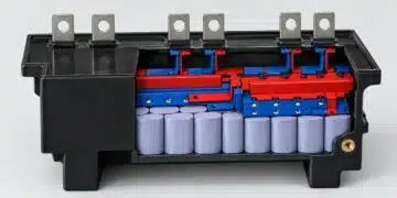




AI server workloads can impose repeated load pulses rather than a steady power demand, particularly when GPUs operate synchronously during training.
Predicting power-supply efficiency under these conditions requires more than a conventional steady-state efficiency curve: semiconductor temperature retains the history of previous load intervals. An illustrative electrothermal model developed by Sam Ben-Yaakov explains how this thermal memory affects losses and how to calculate efficiency over a complete load cycle.
Why steady-state efficiency curves are not enough
A steady-state efficiency curve associates each load point with a thermally settled operating condition. After the load changes, the power supply is allowed to reach a stable temperature before efficiency is recorded.
Pulsed operation follows a different sequence. When the load falls after a high-power interval, the semiconductor junctions and cooling system remain warm. The losses during the following low-power interval therefore need not match those measured at the same load after thermal stabilization. The reverse occurs when the load rises again. A relatively cool junction initially produces lower losses in the temperature-dependent model, but those losses increase as the junction heats.
The central issue is temperature: instantaneous load alone does not determine instantaneous efficiency. Pulse duration, repetition period, cooling conditions and the temperature left by preceding pulses all influence the result. Synchronized GPU activity makes this relevant at system level. Load pulsations from multiple cards can reinforce one another on a shared power rail and propagate upstream. The example establishes the motivation for studying pulsed operation; it does not define a universal AI server load profile.
Operating principle: an electrical model of heat flow
An electrothermal equivalent circuit represents heat generation, heat flow and heat storage using familiar electrical elements.
| Thermal quantity | Electrical representation | Purpose in the model |
|---|---|---|
| Dissipated power | Current source | Injects the calculated losses into the thermal network |
| Temperature | Voltage | Represents junction, heat-sink and ambient temperatures |
| Thermal resistance | Resistor | Represents the restriction to heat flow between thermal nodes |
| Thermal capacitance | Capacitor | Represents stored thermal energy and delayed temperature changes |
The thermal path starts at the MOSFET junction, passes through the package and mounting interface, and continues through the heat sink to ambient. Thermal resistance alone describes the relationship between dissipation and temperature rise after settling. Adding thermal capacitance allows the model to reproduce heating and cooling over time. These capacitors are simulation analogues of heat storage, not physical capacitors added to the power stage.
The simplified example uses two thermal capacitances: one associated with the junction region and another with the heat sink. Their different time constants allow the junction to respond relatively quickly while the heat sink changes temperature more slowly. Illustrative time scales discussed range from a few milliseconds to around 100 milliseconds for transistor or module thermal behaviour, with much longer responses—potentially half an hour or an hour—for large cooling systems. These are examples, not component-selection limits.
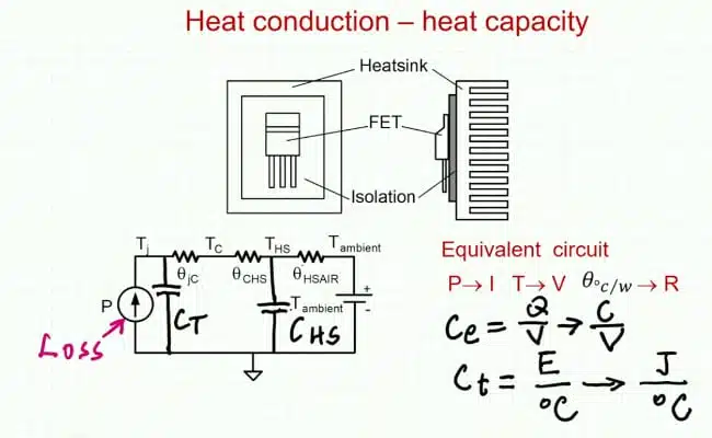
More detailed thermal networks can use multiple stages to represent heat spreading through the semiconductor package and cooling assembly. The two-capacitance network is deliberately retained here to make the interaction between load, losses and temperature easier to follow.
Temperature-dependent conduction and switching losses
The example considers two semiconductor loss mechanisms.
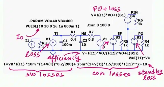
- Conduction losses arise from current flowing through MOSFET on-resistance. The model makes this contribution proportional to the square of the inductor current and to a temperature-dependent effective resistance.
- Switching losses are represented by a behavioural term proportional to bus voltage and current, with a separate temperature dependence.
Both loss contributions increase with junction temperature in the illustrative model. This creates positive electrothermal feedback: higher losses increase temperature, which increases losses further. The analysis flags thermal runaway as a possible consequence of excessive positive feedback, but it does not investigate a runaway condition or establish a stability margin.
A simplified buck-converter representation
The electrical example is based on a buck converter, but it is an averaged behavioural loss model rather than a detailed switching simulation. A single effective on-resistance represents semiconductor conduction losses. This is a simplification: the high-side and low-side devices have different conduction intervals, and their individual contributions require appropriate treatment in a device-level model.
Temperature dependence is approximated with linear scaling. One illustrative conduction-loss coefficient produces a resistance at the upper end of the chosen temperature span that is 2.5 times its value at 0°C. Switching-loss temperature coefficients of 0.2 and 0.5 are discussed for different illustrative settings. These coefficients are assumed demonstration parameters. They are not measured characteristics of an identified MOSFET, a specified server power supply or a particular semiconductor technology.
Illustrative simulation conditions
The behavioural model combines a pulsed current source, temperature-dependent semiconductor losses, a fixed auxiliary-loss term and the thermal network.
| Parameter | Illustrative value | Interpretation |
|---|---|---|
| Input bus voltage | 400 V | Assumed electrical operating point |
| Output voltage | 40 V | Fixed output voltage used in the power calculation |
| Initial current profile | 10 A to 30 A | Low- and high-load levels |
| Load-pulse period | 1 s | Repetition period of the workload envelope |
| High-load interval | 0.8 s | 80% of each load cycle |
| Effective on-resistance reference | 25 mΩ at 0°C | Assumed conduction-loss parameter |
| Switching-loss scaling | 1% of the bus-voltage–current product, before temperature scaling | Behavioural approximation, not an efficiency rating |
| Fixed auxiliary losses | 10 W | Represents overhead such as drivers and auxiliary supplies |
| Ambient temperature | 0°C | Assumed thermal boundary condition |
| Initial transient simulation | 0–100 s | Observation interval, not proof of thermal settling |
| Alternative current profile | 1 A to 30 A | Demonstrates the effect of overhead at lighter load |
The 80% duty cycle describes the high-load portion of the workload envelope. It is not the switching duty cycle of the buck converter. Likewise, the 1% switching-loss factor applies to the bus-voltage–current product used in the model. It should not be interpreted as 1% of output power or as a universal switching-loss allowance. The 0°C ambient is another modelling assumption. Applying the same method to an actual product requires the real thermal boundary conditions and temperature-dependent device data.
How thermal memory changes efficiency during a pulse
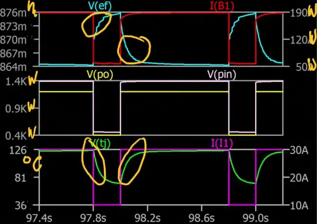
The simulation distinguishes between rapid junction-temperature changes and slower heat-sink warming. During the initial 100-second run, the heat sink has not yet reached a stable temperature.
Within an individual load cycle, the sequence is:
- After the high-load interval, the junction remains hot as the load falls.
- During the low-load interval, cooling reduces the temperature-dependent loss contribution, allowing efficiency to recover.
- At the next high-load transition, the cooler junction initially gives better efficiency.
- As the junction reheats, efficiency decreases towards the value associated with the warmer operating condition.
This is why simply looking up the two load levels on a steady-state efficiency curve does not reproduce the transient behaviour.
Why the low-load level matters
A second example lowers the minimum current from 10 A to 1 A while retaining the 30 A high-load level and the 10 W fixed-loss term. At the lower minimum load, the auxiliary overhead becomes more significant relative to useful output power. Low-load efficiency consequently falls, even though the junction can cool during that interval.
Two effects must therefore be kept separate:
- Cooling can reduce temperature-dependent semiconductor losses.
- Fixed overhead can still dominate efficiency when useful output power is small.
The result is not a general claim that pulsed operation always improves or worsens efficiency. It demonstrates why both the thermal trajectory and the actual low-load consumption must be included.
Calculating average efficiency correctly
For the complete observation interval, average efficiency is calculated from average output power divided by average input power:
In the behavioural model, input power is reconstructed from output power and calculated losses:
This method accounts for the different amounts of power transferred during the high- and low-load intervals. An arithmetic average of instantaneous efficiency values does not implement the calculation used here. For a workload comparison, the input and output averages should cover the same interval. An evaluation intended to represent sustained operation should also distinguish the initial warm-up period from operation after the relevant thermal conditions have settled.
Interpreting the numerical result cautiously
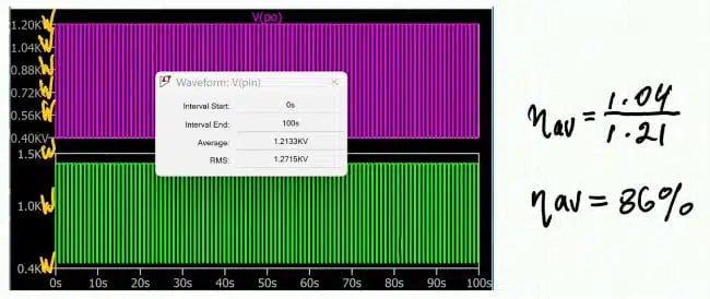
The final demonstration reports average efficiency of approximately 86%, with instantaneous efficiency varying roughly between 85% and 88%. However, the spoken transcript also gives rounded average-power values of approximately 1 kW output and 1.21 kW input. Those values do not reproduce the reported efficiency when used literally. The exact numerical result should therefore be checked against the plotted simulation readouts before being reused as a benchmark. The supported engineering takeaway is the calculation method and its dependence on thermal history—not an independently validated efficiency rating for an AI server power supply.
Design-in notes for engineers
The following points are editorial application guidance based on the model’s scope and limitations, not additional measured results.
- Define the workload envelope. Record both current levels, pulse duration, repetition period and the amount of synchronization between loads.
- Use application-specific loss parameters. Replace the assumed effective resistance, switching-loss scaling and temperature coefficients with validated data.
- Separate warm-up from sustained operation. A repeating current waveform does not establish that the heat sink has reached a repeating thermal condition.
- Include auxiliary consumption. Driver and auxiliary-supply losses can materially affect efficiency during low-load intervals.
- Validate the thermal network. Use thermal data and measurements appropriate to the package, mounting interface and cooling arrangement.
- Keep pulse duty cycle separate from converter duty cycle. They describe different processes and must not be interchanged.
- Do not treat this as a complete passive-component model. The example does not provide a separately validated loss breakdown for inductors, capacitors or filters.
- Qualify components independently. No inductance, saturation-current, DCR, capacitor ripple-current or ESR requirement can be selected from this demonstration alone.
- Compare suppliers under matched conditions. For purchasing evaluations, request pulsed-load results with a defined workload, ambient condition, cooling arrangement and averaging window.
For a broader discussion of model scope and verification, the guide to measuring, modeling and simulating capacitors and inductors provides a useful next step.
Limits and trade-offs
The averaged approach makes electrothermal interactions easier to study without resolving every switching event. It is useful for exploring how pulse profiles, thermal time constants and fixed losses influence calculated efficiency.
That simplicity also limits what can be concluded. The example does not establish switching-frequency ripple, control-loop response, EMI performance or component-level passive losses. It does not identify a complete server power-supply topology or validate the assumed coefficients against hardware.
Adding a more detailed thermal network or separate device-loss models can improve application relevance, but only when supported by appropriate parameters and validation. Increasing model complexity alone does not establish accuracy.
Conclusion
Pulsed-load efficiency requires a coupled view of power loss and temperature. A steady-state curve cannot, by itself, describe a supply whose junctions heat and cool while the cooling assembly continues to warm.
The behavioural method provides a practical framework: apply the load profile, calculate temperature-dependent losses, track the thermal response and obtain efficiency from average output and input power over the same interval. Its numerical predictions remain dependent on the quality of the loss parameters, thermal model and operating conditions.
Further reading
- DC-DC Converter Basic Characteristics and Formulas
- How to Choose the Right Inductor for DC-DC Buck Applications
Source
Adapted from Sam Ben-Yaakov’s technical presentation, “AI servers Power supply: efficiency under pulsed load,” published on 3 November 2026. The numerical conditions are illustrative simulation assumptions, not specifications or measured performance of a commercial server power supply.
The introductory GPU-load example refers to a study whose bibliographic details are not established by the available transcript; no additional findings from that study are used here. Suggested figure timestamps identify the relevant discussion points. Confirm the exact frame and legibility before capturing publication screenshots.
References
- Original technical presentation and transcript: AI servers Power supply: efficiency under pulsed load — Sam Ben-Yaakov.