B–H Curve-Based Inductor Modelling in LTspice: A Current-Dependent Magnetic Model

Accurate inductor simulation becomes difficult when a ferrite core approaches saturation, because inductance is no longer constant and the local slope of the B–H curve changes sharply.

In this presentation, Sam Ben-Yaakov introduces a B–H-table-based LTspice model intended to represent the current-dependent behaviour of a gapped ferrite inductor more directly than a conventional fixed-reluctance approach.

Why this topic matters

Power inductors in switching converters operate with DC bias plus ripple current. As current rises, the magnetic material can enter its nonlinear region, reducing inductance and potentially increasing ripple current, peak switch current, losses, and thermal stress.

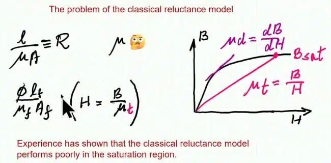
A conventional magnetic-circuit model is useful for first-order design, particularly where the material can be approximated by a constant permeability. However, treating permeability as a fixed quantity becomes problematic close to saturation, where the B–H relationship is nonlinear and the distinction between total and differential permeability becomes important.

For broader context, see saturation current of inductors and its measurement and LTspice inductor modelling methods.

Operating principle

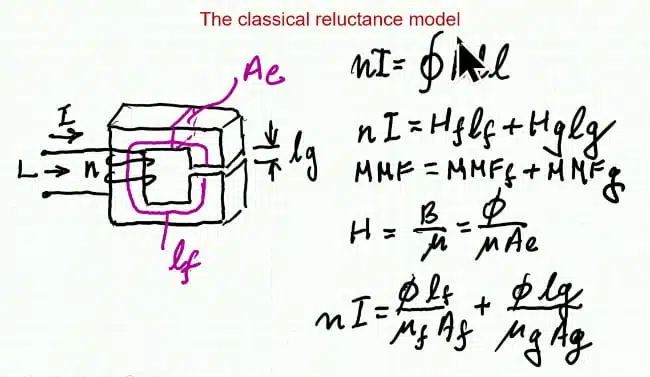
The classical reluctance approach starts from Ampère’s law:

$NI = \oint H\,dl$

For a simple gapped magnetic structure, the magnetomotive force is divided between the ferrite path and the air gap. With flux density expressed as flux divided by effective core area, the magnetic circuit can be represented through reluctances:

$\mathcal{R} = \frac{l}{\mu A_E}$

In the electrical analogy used in the presentation:

• Magnetic flux is represented by electrical current
• Magnetomotive force, NI, is represented by voltage
• Magnetic reluctance is represented by electrical resistance
• The ferrite and air-gap reluctances appear as series elements in the equivalent circuit

This analogy is particularly convenient for circuit simulation because it lets the magnetic structure interact with electrical excitation in a SPICE environment.

An air gap is commonly used in a power inductor because it raises total magnetic reluctance and provides energy-storage capability. It also lowers effective permeability, allowing the magnetic assembly to handle greater DC bias before the ferrite reaches deep saturation. The trade-off is lower inductance for a given core and turns count, as well as gap fringing that can increase winding AC loss. See how gapped cores manage saturation and energy storage.

Permeability is not one quantity

The presentation highlights a key modelling issue: total permeability and differential permeability should not be treated as interchangeable.

Total permeability is based on the ratio of flux density to magnetic-field strength:

$\mu_\mathrm{total} = \frac{B}{H}$

Differential, or small-signal, permeability is based on the local slope of the B–H curve:

$\mu_\mathrm{diff} = \frac{dB}{dH}$

In the approximately linear region of a ferrite B–H curve, both values are similar. Near saturation, their behaviours diverge: total permeability can decrease relatively gradually, while differential permeability can collapse much more sharply as the B–H curve flattens.

This distinction matters because a converter responds to incremental inductance at its instantaneous operating current. A small current perturbation around a high DC bias does not necessarily see the same inductance as a large-signal ratio calculated from total flux and current.

Modified B–H model

Instead of representing the ferrite with a fixed reluctance, the proposed method uses a current-dependent source whose value is derived from the material’s B–H data.

The model workflow is:

1. Measure the voltage representing the magnetomotive force across the ferrite element.
2. Divide this quantity by ferrite magnetic path length to obtain magnetic field strength.
3. Use a table of B–H pairs to determine the corresponding flux density.
4. Multiply flux density by effective core area to obtain magnetic flux.
5. Represent the resulting magnetic flux as the current of a dependent source in the electrical analogue.

The central relationship is:

$\Phi = B \cdot A_E$

The B–H characteristic is therefore entered as a lookup table, rather than reconstructed from a single constant-permeability term. The presentation uses a B–H curve taken from the Ferroxcube 3C90 ferrite material data, extracting an averaged B–H relationship from the hysteresis-loop plot.

The air gap remains well suited to the conventional reluctance representation because its permeability is effectively that of air and can be treated as constant for this first-order model.

LTspice implementation

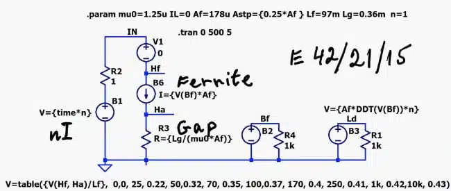
The example uses LTspice behavioural sources and the table function. The voltage across the ferrite modelling element is divided by the ferrite magnetic path length to obtain the input to the B–H table.

The table returns the corresponding flux density. Multiplication by the effective core cross-sectional area produces the modelled flux, represented in the electrical analogue as dependent-source current.

The presentation stresses that the excitation source is defined as a function of time. This makes it possible to derive local properties in the time-domain simulation by relating the imposed current sweep to time.

The model requires the following input data:

• Effective core cross-sectional area
• Ferrite magnetic path length
• Air-gap length, if applicable
• Number of winding turns
• A usable B–H data set for the selected material
• An LTspice lookup-table implementation of the B–H characteristic

A practical limitation is the quality of the B–H input data. A curve digitised from a datasheet plot is suitable for exploratory modelling, but it may not reflect production spread, temperature, excitation frequency, DC premagnetisation, mechanical gap tolerance, or the exact waveform in the intended converter.

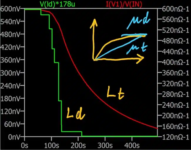
Total and differential inductance

The presentation defines total inductance as flux linkage divided by current:

$L_\mathrm{total} = \frac{N\Phi}{I}$

This quantity describes the overall large-signal relationship at a particular operating point. In contrast, local or differential inductance is the incremental change in flux linkage with current:

$L_\mathrm{diff} = N\frac{d\Phi}{dI}$

The model derives local inductance from the time-domain derivative because the excitation current is made proportional to simulation time. In LTspice, a derivative function can therefore be applied to the reconstructed B–H-dependent flux signal.

The video shows that total inductance and differential inductance coincide in the linear region. As saturation is approached, differential inductance falls much more abruptly, whereas total inductance decreases more gradually.

Quantity	Definition	Design meaning near saturation
Total inductance	$N\Phi/I$	Describes the large-signal flux-current relationship at an operating point
Differential inductance	$N(d\Phi/dI)$	Indicates incremental current response and is often more relevant to ripple and loop dynamics
Constant inductance assumption	A single fixed L value	Acceptable only when the operating range remains sufficiently linear

Video example

The simulation example uses an E-core identified in the presentation as E 42/21/15 with a 0.36 mm air gap. For the linear operating region, the simulation produces approximately 600 nH.

The presentation compares this result with a stated measured value of 630 nH for the same 0.36 mm gap condition. The presenter describes the agreement as good for a theoretical, first-order calculation.

This numerical comparison should be treated as an illustrative validation point rather than a guaranteed prediction method. The video does not provide the complete measurement setup, winding details, temperature, test frequency, flux level, instrument method, or mechanical-tolerance information needed to generalise the result to another design.

Video-provided example	Value stated in presentation
Core family	E 42/21/15
Air-gap length	0.36 mm
Simulated inductance in linear region	Approximately 600 nH
Referenced measured inductance	630 nH

Behaviour without an air gap

The presenter also removes the air-gap reluctance from the model to examine the ferrite material on its own. In this configuration, the reconstructed B–H curve closely follows the B–H data used to populate the lookup table.

This acts as a consistency check: if the model reproduces the selected relationship between flux density and magnetic field, then total inductance and differential inductance follow from that relationship and the known core geometry.

An ungapped ferrite core reaches nonlinear operation at lower current than a comparable gapped power inductor. That can be appropriate for transformers, current transformers, or resonant magnetic components when the flux excursion is controlled, but it is generally less forgiving in an energy-storage inductor carrying a significant DC component.

Design-in notes for engineers

• Use the B–H curve applicable to the intended ferrite material, and treat digitised plot data as an approximation unless the supplier provides validated numerical data.
• Model both DC bias and peak-to-peak ripple current, because saturation risk is set by instantaneous peak current rather than nominal DC current alone.
• Inspect differential inductance as well as total inductance when assessing current-loop stability, current-mode control behaviour, peak-current limit margin, and ripple-current prediction.
• Include the air gap explicitly for energy-storage inductors, since it often dominates effective reluctance and strongly affects inductance and DC-bias capability.
• Account separately for winding DCR, frequency-dependent AC resistance, core loss, parasitic capacitance, and thermal rise; the presented model is focused on the nonlinear flux-current relationship.
• Validate gap length and assembly tolerance. Small differences in effective air gap can create substantial inductance variation, especially where the gap dominates the magnetic circuit.
• Keep windings and conductive hardware clear of high-fringing-field regions near discrete gaps; fringing-field loss modelling in inductors and transformers provides further context.
• Correlate simulation with bench measurements over current and temperature, rather than relying on one low-current inductance measurement.

Limits and trade-offs

The presenter explicitly characterises the approach as a first-order approximation. It does not account for leakage flux, air-gap fringing, or non-uniform flux-density distribution within the ferrite.

The model also relies on an averaged B–H relationship. It is therefore not a complete hysteresis-loss model, nor does the presentation establish a method for predicting core loss over waveform, frequency, and temperature.

Finite-element analysis can add important geometric detail, especially for gap fringing, local saturation, winding fields, and complex core geometry. However, the presentation cautions that FEA results are only as reliable as the B–H model and material data entered into the solver.

Approach	Main strength	Important limitation
Constant-reluctance model	Fast, simple, useful in a linear region	Cannot directly capture nonlinear B–H behaviour near saturation
B–H-table dependent-source model	Represents a selected nonlinear B–H curve in circuit simulation	First-order model; excludes leakage, fringing, spatial flux distribution, and loss mechanisms
Finite-element analysis	Can resolve geometry-dependent field distribution	Still depends on valid material data, boundary conditions, and modelling assumptions

Practical applications

The proposed modelling approach is most relevant where inductance changes materially over the intended current range:

• Buck and boost converter output inductors
• Active PFC boost inductors
• High-current point-of-load converters
• Energy-storage chokes in isolated DC/DC converters
• Current-dependent inductors used intentionally for nonlinear magnetic behaviour
• Magnetic design exploration before detailed prototype measurement
• Circuit-level studies of current ripple, peak current, and saturation-related operating shifts

For purchasing and component qualification, the model also reinforces why a single nominal inductance value is insufficient. Relevant supplier data should include inductance-versus-current characteristics, temperature conditions, saturation-current definition, DCR, thermal-current rating, core material, and test method.

Further reading

The video is identified as the second part of a three-part sequence on current-dependent inductors. The first video covers an overview and applications, while the planned third part is intended to examine the design of inductors with deliberately tailored current dependence, including stepped air-gap concepts.

For a complementary portal resource, see current-dependent inductor modelling and the LTspice inductor riddle.

Source

This article adapts the technical presentation by Sam Ben-Yaakov, “A modified BH-based electromagnetic elements model.” The presentation describes a current-dependent, B–H-table-based LTspice approach for modelling nonlinear ferrite magnetic elements and compares total with differential inductance.

References

• Sam Ben-Yaakov, A modified BH-based electromagnetic elements model
• Passive Components Blog, Saturation Current of Inductors and its Measurement
• Passive Components Blog, Inductors Modeling with LTspice
• Passive Components Blog, Understanding Inductors With Gapped Cores
• Passive Components Blog, Modeling Fringing Field Losses in Inductors & Transformers