How to Measure Filter Performance: Insertion Loss, VNA Fixtures and CM/DM Separation

A filter insertion-loss curve is only useful when the measurement setup, reference planes and source and load impedances behind it are known, and when the result is translated into the impedances of the real application.

This guide joins the measurement topics of the Passive Components Blog filter series into one bench workflow. It assumes the definitions from the filter S-parameters article and the introduction to insertion loss and filter capacitor performance and focuses on how to measure a filter with a vector network analyzer (VNA), how to separate common-mode (CM) and differential-mode (DM) noise in a conducted-emissions setup, and how to interpret the results. Component suppliers such as Würth Elektronik publish mixed-mode measurement data and fixture details that follow the same principles [1]. A worked example based on a published power inlet filter measurement shows the complete workflow with documented setup and before/after results [2], [3].

Key Takeaways

• A VNA measures the small-signal transfer function of an unpowered filter between defined impedances, while a conducted-emissions setup measures the noise of the powered equipment through a LISN. Both are needed, and they answer different questions.
• Calibrate at the point where the fixture meets the filter, or de-embed the fixture, and verify the reference planes with a known component before trusting a result.
• A 50 Ω/50 Ω curve is a comparison value. In real terminations the same filter can lose tens of decibels or show insertion gain at its LC resonance [4].
• Separate CM and DM noise before designing or modifying a filter, because each filter section attenuates mainly one mode.
• Mains LISNs carry high protective-earth currents and expose the receiver to transients: bond the protective earth first, use an isolation transformer and protect the analyzer input [5].

VNA or Conducted-Emissions Setup: What Each Measurement Answers

Filter measurements fall into two groups. The first characterizes the filter itself as a two-port or four-port network: the VNA drives a small sinusoidal signal through the unpowered filter and measures S21 between defined reference impedances. The second measures the noise that the powered equipment injects into a line impedance stabilization network (LISN), with and without the filter. The conducted-emissions line filter webinar covers the second group in more detail; Table 1 compares both.

Aspect	VNA insertion loss (component measurement)	Conducted emissions with LISN (system measurement)
Question answered	How much does the filter attenuate between defined impedances?	Does the equipment with this filter meet the limit, and which mode dominates?
Stimulus	VNA source, typically 0 dBm to +13 dBm, swept sine	The equipment’s own switching noise
Terminations	50 Ω, or CISPR 17 alternatives such as 0.1 Ω/100 Ω	LISN on the line side (50 Ω per line); real equipment on the other side
Operating state	Unpowered, no load current and no line voltage	Rated voltage and load current; chokes and capacitors under bias
Typical range	Bode 100 class: 1 Hz to 50 MHz; RF VNAs to GHz	9 kHz or 150 kHz to 30 MHz (CISPR 25 voltage method to 108 MHz)
Mode information	CM and DM measured separately by connection or with baluns	V1 and V2 per line; CM and DM by calculation, combiner or separator
Main limitation	Ignores source and load impedance, bias and installation coupling	Result is valid only for this equipment, layout and operating point
Best use	Comparing filters, checking a sample against its datasheet, building models	Pre-compliance, choosing the filter section to change, before/after checks

The VNA measurement uses the CISPR 17 insertion-loss definition: the ratio of the load voltage without and with the filter for a given source impedance Z_S and load impedance Z_L [8]. Written with the ABCD (chain) parameters of the filter, the definition shows directly why the result changes with the terminations:

Here V_L0 is the load voltage without the filter and V_L is the load voltage with the filter. For Z_S = Z_L = 50 Ω, Eq. (1) equals −20 log₁₀|S21|. The same equation, evaluated with the measured or modelled filter and the application impedances, is used later in the worked example.

Reference Planes, Fixtures, Calibration and De-Embedding

A VNA is calibrated at its coaxial interface, the measurement plane, while the filter performance is needed at the point where the component attaches to the board, the device plane. Anything between the two planes, such as cables, adapters, PCB traces and pads, becomes part of the result unless it is calibrated out or removed mathematically [9].

Choose the connection method by frequency

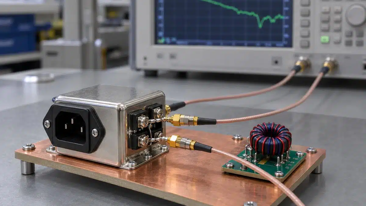
Below about 30 MHz, short coaxial connections soldered directly to the filter terminals are usually sufficient. In the OMICRON Lab power inlet filter measurement, connecting the filter with test grabbers produced a resonance at about 28 MHz that did not belong to the filter; BNC connectors soldered close to the terminals removed it [2]. A 0.5 m RG58 cable alone has about 45 pF and 150 nH of parasitics, and calibration standards themselves are not ideal: a BNC thru connector adds about 1 pF and a shorting bar about 1 nH [6]. For SMD filters, a PCB fixture with controlled-impedance traces, as described in the PCB fixtures and solder-wick article, keeps the fixture repeatable.

Calibrate, extend or de-embed

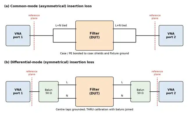
• Calibrate at the fixture: perform the SOLT or THRU calibration with the standards placed where the filter will be connected. For the DM measurement, join the two baluns directly for the THRU calibration so that the baluns are calibrated out [2].
• Include the fixture in the calibration: CMC test specifications for automotive Ethernet define the calibration reference at the CMC pads of the test board, with 50 Ω ±5 Ω traces and at least 10 samples per test [10].
• Port extension: fast and adequate when the fixture is a short, well-matched line; it compensates delay and loss but not mismatch.
• De-embedding: measure or model the fixture halves and remove them with T-parameter matrices, either in post-processing or inside the VNA calibration for real-time display [9].

Fixture layout is part of the result at high frequencies. In Würth Elektronik measurements of ceramic common-mode filters, a via-in-pad layout degraded the common-mode insertion loss by up to 5 dB compared with layouts that had symmetric return paths, and one layout produced measurement artifacts that were attributed to the fixture rather than to the filter [1].

Low impedance: shunt-through and the ground loop

Filter capacitors, feedthroughs and power rails are characterized as impedances in the milliohm range. The two-port shunt-through method, described in the shunt-through power integrity article, converts S21 into impedance, and series-through is used for high impedances such as choke impedance:

The optimum range is about 1 mΩ to 100 Ω for shunt-through and about 1 kΩ to more than 1 MΩ for series-through on a Bode 100 class analyzer [6]. In shunt-through, the internally connected grounds of the VNA ports form a ground loop. A 2 mΩ resistor measured 6.855 mΩ at 1 kHz without correction and 2.215 mΩ with a common-mode choke in the cable, while both readings agreed at 100 kHz [6]. A modelled DC case showed an error of nearly 460 % from the same loop, which is why a 50 Ω common-mode transformer or a semi-floating differential amplifier is inserted for milliohm measurements [11]. The capacitor and inductor measurement article lists the method choice by impedance range.

Interpreting 50 Ω Results for a Real Application

A 50 Ω/50 Ω insertion-loss curve is easy to measure and reproducible, so datasheets use it for comparison. A power line filter, however, works between the mains impedance and the input of a converter, and both change with frequency. Schaffner compared 50 Ω curves with noise measurements in real equipment: 50 Ω curves consistently overestimated the effective attenuation, and a prediction based on them deviated by up to 20 dB at low frequencies, whereas a prediction based on the CISPR 17 approximate worst-case curves matched the real noise almost exactly below 10 MHz [4].

The CISPR 17 approximate worst-case method measures the filter with 0.1 Ω on one side and 100 Ω on the other, then repeats the test with the terminations reversed [4]. Because a purely resistive 0.1 Ω is difficult to realize over frequency, 1 Ω/100 Ω is used as a nearly worst-case substitute; one published example filter showed 30 dB common-mode insertion loss at 1 MHz in 50 Ω but only about 0.9 dB in 0.1 Ω/100 Ω [12]. The article on EMC filters for real operating environments shows how an L-section loses about 50 dB when its capacitor faces the low impedance.

Effect	What the 50 Ω curve hides	Practical check
Source and load impedance	Mismatch between filter sections and terminations; LC resonance and insertion gain	Evaluate Eq. (1) with CISPR 17 or estimated application impedances
Filter orientation	Y capacitors on the line side can create a dip; Schaffner observed one at 6 MHz	Measure both orientations and keep the capacitors on the high-impedance side
Load current	Choke inductance falls with peak current; up to 50 % loss of inductance allows about 6 dB lower attenuation	Measure the peak line current and compare it with the choke saturation curve [4]
DC and AC bias	Ceramic capacitance and ferrite impedance drop under bias	Repeat the measurement with a bias tee or use bias-dependent models
Temperature and tolerance	CMC inductance can fall by 20 % to 40 % at low temperature	Add design margin or measure over temperature
Installation coupling	Above about 10 MHz, coupling across the filter can bypass it [4]	Verify in the enclosure with the final wiring and grounding

Bias effects are often larger than the measurement uncertainty. Ferrite beads lose a large part of their impedance under DC current, as shown in the DC bias study of SMT EMI suppression ferrites, and common-mode chokes in the 800 V DC EMC filter guide carry a ±30 % tolerance with a further 20 % to 40 % inductance drop at low temperature in worst cases.

CM/DM Separation and Balanced Interfaces

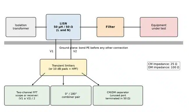
A LISN does not measure CM and DM noise directly. It measures the noise voltages V1 and V2 of the two supply conductors across 50 Ω, and each contains both modes [13]. The modes are obtained by addition and subtraction:

The CM noise sees the two 50 Ω LISN resistors in parallel, 25 Ω, while the DM noise sees them in series, 100 Ω. These are the impedances to use when the filter attenuation is evaluated for each mode. Some separators define V_DM as V1 − V2 without the factor of one half, so the convention must be checked before comparing results [14].

Method	How it works	Accuracy and range	Notes
Two-channel FFT math	Record V1 and V2 at the same time and compute Eq. (4)	Depends on channel matching and phase; 9 kHz RBW in the 800 V example	Low cost; used in the 800 V DC filter guide
0°/180° combiner	0° combiner gives V1 + V2, 180° combiner gives V1 − V2	Mini-Circuits ZFSC types used from 1 MHz to 108 MHz; error grows below 1 MHz	Correct for combiner loss and subtract 6 dB [13]
CM/DM separator (LISN mate)	Passive network with separate CM and DM outputs	Nominal 150 kHz to 100 MHz; about 42 dB to 55 dB rejection of the other mode from 150 kHz to 30 MHz	Terminate the unused port in 50 Ω; max. 27 dBm and 30 mA DC [14]
VNA with baluns	Inject a pure CM or DM signal into the unpowered filter	Balun bandwidth, e.g. 10 kHz to 80 MHz	Measures filter insertion loss per mode, not equipment noise [2]

Separated results answer the most important design question: which filter section to change. Below about 1 MHz, the noise of a typical switched-mode power supply is mostly differential, and above 1 MHz the common-mode path dominates [4], [13]. The 800 V DC guide uses this to set different targets, about 60 dB CM and 40 dB DM at 300 kHz, instead of designing both sections for the same value.

Balanced data and signal interfaces

For balanced interfaces, common-mode filters and chokes are measured with a four-port VNA and the single-ended S-parameters are converted into mixed-mode parameters. With physical ports 1 and 2 forming the input pair and ports 3 and 4 the output pair, the differential transmission and the common-mode rejection are:

Sdd21 describes the loss of the wanted differential signal, Scc21 the common-mode rejection, and Ssd21 or Scd21 the mode conversion that turns signal into common-mode noise. The OPEN Alliance test specification for 100BASE-T1 chokes, for example, recommends a common-mode rejection of at least 45 dB from 10 MHz to 80 MHz and a differential insertion loss of no more than 0.5 dB up to 10 MHz [10]. A single-ended setup on an application that is balanced can introduce imbalance and artifacts, so baluns or true differential stimulus are recommended for spectrum-based checks [1]. Construction details of the chokes themselves are in the toroids and current-compensated chokes article.

Measurement Limitations and Safe Equipment Connections

Most filter measurement errors come from the setup, and most equipment damage happens at the receiver input. The following rules apply to both bench methods.

LISN and mains safety

• A CISPR 16-1-2 mains LISN has large capacitances from line and neutral to protective earth, so it draws a high leakage current that trips residual-current devices and can be lethal if the earth connection is missing. Its design cannot meet EN 61010-1 [5].
• Bond the LISN ground to the site protective earth before any other connection, and do not remove it until the mains supply is disconnected. Never defeat the protective earth to stop an RCD from tripping.
• Supply the LISN through an isolation transformer rated for the full load current, and only let qualified staff operate the setup [5].
• For high-voltage DC systems, a low-voltage isolated noise source, as used in the 800 V DC guide, allows the filter to be evaluated without a live high-voltage system.

Receiver and VNA protection

• Use a transient limiter or a 10 dB attenuator with a high-pass filter between the LISN and the analyzer. A typical limiter covers 9 kHz to 30 MHz with 10 dB in-band loss and accepts 4 W (+36 dBm) CW [15].
• Spectrum analyzer inputs are typically rated at +20 dBm to +30 dBm. Disconnect the coaxial cable or set the LISN output to off before switching the equipment on or off [5].
• Low-cost analyzers may not present 50 Ω at 50 Hz, which can leave tens of volts of mains residue at an unterminated LISN output; a 9 kHz or 150 kHz high-pass filter prevents this [5].
• Terminate every unused LISN or separator output in 50 Ω, for example the second LISN in a CISPR 25 voltage-method setup [7], [14]. The 48 V automotive EMI article shows CISPR 25 measurements in practice.
• Never connect a VNA port to an energized filter. Discharge X capacitors before connecting, and use a DC block or series resistors, with the corresponding correction, when a bias is applied [6].

Know the limits of the result

A VNA measurement is a small-signal measurement of a single sample at room temperature. It does not include choke saturation, capacitor DC bias, self-heating or coupling inside the final enclosure. A conducted-emissions result is only valid for the measured equipment, cable layout and operating point. Report the instrument, calibration, fixture, terminations, frequency points, resolution bandwidth and the operating state with every result so that it can be repeated.

Worked Example: Power Inlet Filter from Bench to Application

The example combines a published, fully documented VNA measurement of a single-phase power inlet filter [2] with a component model of the same filter derived from measured impedances [3]. The model is then evaluated with Eq. (1) in the 50 Ω setup and in estimated application impedances. The application curves are calculations by the author, not measurements.

Step 1: documented setup

Item	Setting
Analyzer	Bode 100 VNA, transmission/reflection mode, CH2 input 50 Ω
Source level, attenuators	0 dBm; receiver attenuators 20 dB
Receiver bandwidth, points	1 kHz; 401 points
CM connection	Line and neutral tied at each side; BNC connectors soldered close to the filter
DM connection	Two 50 Ω baluns (10 kHz to 80 MHz) soldered to the filter; centre taps grounded
Calibration	THRU calibration at the filter connection points; baluns joined for the DM THRU
Datasheet minimum, CM	14, 23, 30, 41, 45, 50 dB at 0.15, 0.5, 1, 5, 10, 30 MHz
Datasheet minimum, DM	3, 15, 20, 31, 35, 34 dB at the same frequencies

Step 2: fixture before and after

Before: with test grabbers, the measured CM insertion loss showed a resonance at about 28 MHz and did not match the datasheet. After: with BNC connectors soldered to the terminals and a THRU calibration at the same points, the CM insertion loss exceeded the datasheet minimum over the whole range. The DM measurement showed an unexpected peak of 47 dB at 2.2 MHz [2]. An impedance measurement of the input circuit traced the peak to the series resonance of the 104.46 nF X capacitor with 56 nH of inlet inductance and 76.9 mΩ ESR [3].

Step 3: model check in 50 Ω

The model uses the measured element values: common-mode inductance 0.964 mH with 3.81 kΩ parallel resistance and 2.2 pF winding capacitance, a total DM leakage inductance of 3.9 µH, two 2.99 nF Y capacitors with 0.3 Ω ESR and the X capacitor described above [3]. In 50 Ω, the model gives a DM peak of 47.9 dB at 2.2 MHz, in agreement with the 47 dB measured, and exceeds every datasheet minimum, which confirms that the model can be used for the next step.

Step 4: application impedances and the DM resonance

For the application, CM noise is assumed to come from a switching node through 100 pF of parasitic capacitance into the 25 Ω CM impedance of the LISN, and DM noise from a bulk capacitor with 0.1 Ω ESR and 20 nH ESL into the 100 Ω DM impedance. These are illustrative assumptions for a small offline power supply. In the DM path, the 3.9 µH leakage inductance and the X capacitor form a lightly damped resonance:

With a low-impedance DM source, nothing damps this resonance, and the calculated insertion loss becomes an insertion gain of 18 dB at 247 kHz, a case that the 50 Ω curve, with 12.6 dB of loss at 250 kHz, does not reveal. Schaffner reports that such DM insertion gain occurs relatively often in practice [4]. The correction is an RC damping branch across the X capacitor with a resistance close to Z₀; the DC/DC input filter article uses the same principle. A 3.3 Ω resistor in series with a 0.68 µF X2 capacitor removes the gain above 150 kHz and dissipates only about 8 mW at 230 V, 50 Hz.

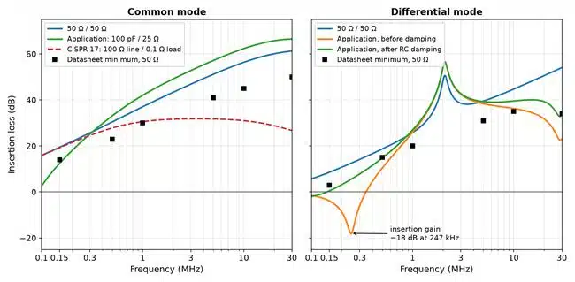
Frequency (MHz)	Datasheet min., 50 Ω (dB)	Model, 50 Ω (dB)	Application, 100 pF/25 Ω (dB)	CISPR 17, 100 Ω line/0.1 Ω load (dB)
0.15	14	19.4	12.4	19.2
0.5	23	30.5	33.1	27.8
1	30	37.1	42.0	30.6
5	41	51.2	57.2	31.8
10	45	56.4	62.4	31.0
30	50	61.3	66.5	26.7

Frequency (MHz)	Datasheet min., 50 Ω (dB)	Model, 50 Ω (dB)	Application before damping (dB)	Application after damping (dB)
0.15	3	8.6	−3.9	0.5
0.25	–	12.6	−17.9	5.7
0.5	15	18.7	10.4	14.7
1	20	25.8	26.0	27.0
5	31	39.5	38.4	39.3
10	35	44.7	36.3	39.6
30	34	54.1	23.2	33.8

What the example shows

• The fixture changed the measured result more than the filter tolerance: one connection method produced a false resonance at 28 MHz.
• The 50 Ω curves met the datasheet, yet the application DM loss at 250 kHz was 30 dB worse than the 50 Ω value, and the CM loss in the 100 Ω/0.1 Ω condition fell to about 27 dB at 30 MHz instead of 61 dB.
• In the assumed application, the CM loss is higher than in 50 Ω above about 0.3 MHz because the high-impedance source and the Y capacitors form a current divider; a low-impedance CM source would reverse this.
• Damping, not more inductance, solved the DM problem. A conducted-emissions measurement with CM/DM separation before and after the change is the final check.

Measurement Checklist

• Define the question: component comparison (VNA) or system compliance (LISN).
• Reference planes: calibrate at the filter terminals or de-embed the fixture; check with a known resistor or C0G capacitor.
• Connections: short coaxial or PCB fixture; no grabbers or long leads above a few MHz.
• Modes: measure CM and DM separately and keep both orientations of the filter.
• Terminations: add CISPR 17 worst-case or application impedances to the 50 Ω result.
• Bias: record DC or AC bias, load current and temperature; compare with saturation data.
• Safety: protective earth first, isolation transformer, transient limiter, 50 Ω terminations on unused ports.
• Documentation: instrument, calibration, IF or resolution bandwidth, source level, fixture photo and operating state.

Conclusion

Filter measurement is reliable when the reference planes are defined by calibration or de-embedding, when CM and DM are measured separately, and when 50 Ω results are treated as comparison values rather than as predictions. The VNA characterizes the filter, the LISN-based conducted-emissions setup verifies the equipment, and the insertion-loss equation with source and load impedances connects the two.

The worked example shows that a filter which meets its 50 Ω datasheet can still lose most of its low-frequency DM attenuation, or even amplify noise, in its application. Checking the result in worst-case or estimated impedances, damping resonances and confirming the change with a separated before/after emission measurement turn a datasheet curve into a usable design result. The filter technology selection guide helps choose the filter type before it reaches this measurement stage.

FAQ

How to Measure Filter Performance

Further Reading

• Introduction to EMI Filtering: insertion loss, filter types and selection.
• Five Key Filter Specifications: the parameters that measurements must confirm.
• AC Line Filter Calculation, Design and LTspice Simulation: modelling CM and DM filter sections.
• EMC Filters Explained: From Component to Design: chokes, capacitors, layout and testing.
• 3-Phase EMI Filter Design, Simulation, Calculation and Test: measurement of three-phase filters.
• Bypass Capacitor S-Parameter Models: how fixture and mounting affect capacitor data.
• ESR of Capacitors: measurement of capacitor losses that damp filter resonances.
• Improving Common Mode Noise Reduction: CM noise paths and stitching capacitors.

References

1. S. Banik, R. Schillinger, S.-M. Wacker, ANP093: WE-CCMF Ceramic Common-Mode Filters for EMI Suppression and Signal Integrity in High-Speed Differential Interfaces, Würth Elektronik, 2026.
2. F. Hämmerle, B. Mößlang, RFI Power Inlet Filter Insertion Loss Measurement, OMICRON Lab application note V2.1, 2016.
3. B. Mößlang, EMC Filter Insertion Loss Simulation, OMICRON Lab application note V2.1, 2022.
4. CISPR 17 Measurements: 50 Ω/50 Ω versus 0.1 Ω/100 Ω, a practical study using the FN 9675-3-06 power line filter, Schaffner EMV AG, 1996.
5. TBL5016-2C 50 µH AC-LISN manual, Tekbox, V1.1, 2025.
6. T. Schuster, F. Hämmerle, Impedance Measurements using the Bode 100, OMICRON Lab application note V1.2.
7. M. Eaker, D. Berger, Understanding CISPR25 Current Probe and Voltage Method for Conducted Emissions, Texas Instruments, SLLA569B, 2025.
8. M. Zhang, Insertion Loss and Filter Performance, Interference Technology, March 2022.
9. De-Embedding and Embedding S-Parameter Networks Using a Vector Network Analyzer, Keysight Technologies, application note 5980-2784.
10. B. Körber, 100BASE-T1 EMC Test Specification for Common Mode Chokes, OPEN Alliance, v2.0, 2020.
11. A. Davis, S. Sandler, The 2-Port Shunt-Thru Measurement and the Inherent Ground Loop, Signal Integrity Journal, April 2019.
12. J. Dřínovský et al., Insertion Loss Estimation of EMI Filters in Unmatched Input/Output Impedance System, Radioengineering, vol. 20, no. 1, 2011, pp. 295–298.
13. L. Jiang et al., A Practical Method for Separating Common-Mode and Differential-Mode Emissions in Conducted Emissions Testing, Analog Dialogue, vol. 55, January 2021.
14. TBLM2 LISN-Mate CM/DM separator manual, Tekbox, V1.3, 2026.
15. LIT-930A transient limiter for conducted emissions testing, Com-Power.
16. Würth Elektronik – EPCI premium supplier page, Passive Components Blog.

Article written and technically reviewed in November 2026