Passive Filter Technologies Compared: LC, Ferrite, Feedthrough, Ceramic, Cavity, Microstrip, SAW and BAW

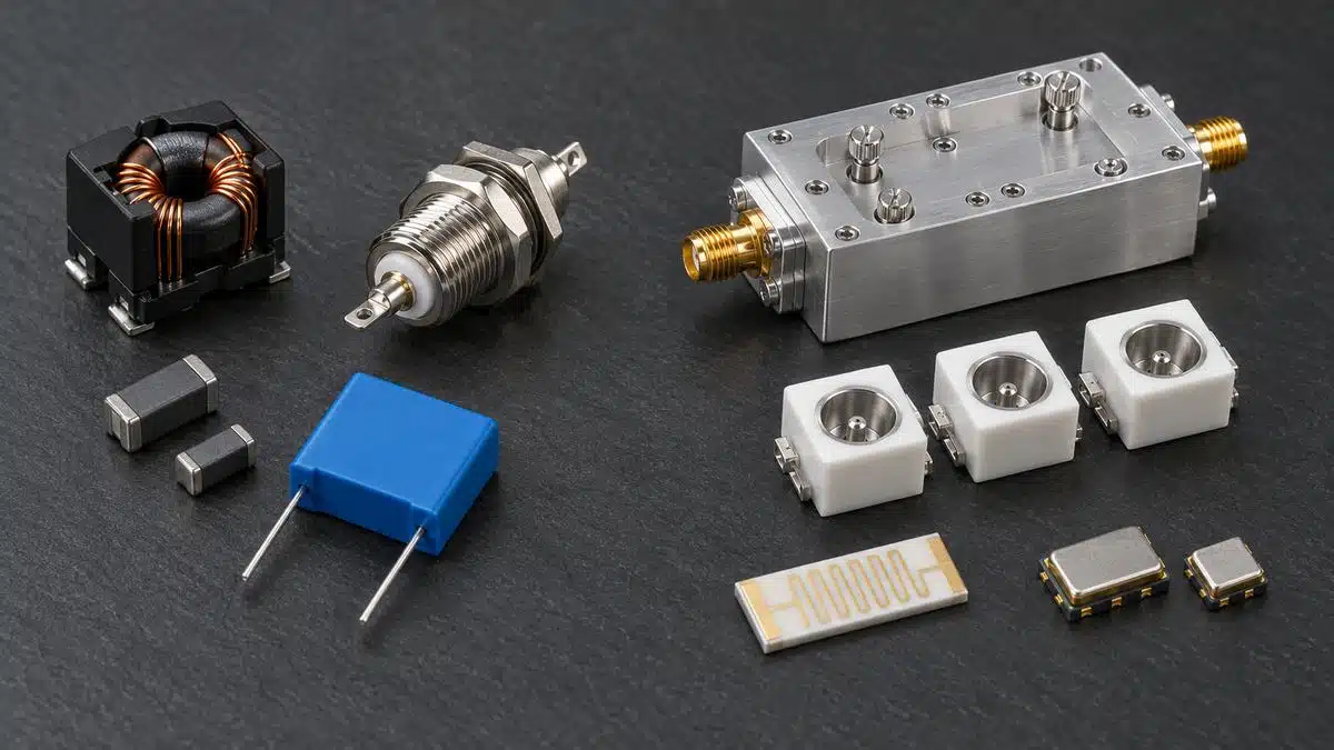
Choosing a passive filter technology starts with one question: is the filter meant to keep unwanted energy out of a power or signal line, or to select a wanted RF band from a crowded spectrum?

This guide separates these two problems and compares LC, ferrite, feedthrough, ceramic, cavity, microstrip, SAW and BAW filters only against the criteria that matter within each application.

This guide connects technical basis draws on design notes from Knowles Precision Devices, Murata, Mini-Circuits, Qorvo, Analog Devices and peer-reviewed reviews, which are listed at the end. The comparison criteria are frequency, bandwidth, insertion loss, selectivity, power or current, size, temperature stability and cost. The numbers quoted are typical values from catalogues and reviews, not limits of any single part.

Key Takeaways

• Decide first whether the task is EMI suppression on a power, supply or I/O line, or RF signal selection in a 50 Ω signal path. The two branches use different specifications, and their technologies are rarely interchangeable.
• EMI filters are judged by attenuation in the real, often unknown, source and load impedances, by current and saturation behaviour, voltage and safety ratings, and by how well the filter is grounded. Insertion loss quoted in a 50 Ω system is only a starting point.
• RF signal filters are judged by insertion loss, selectivity, bandwidth, power handling, temperature drift and size. Unloaded resonator Q and fractional bandwidth together set the minimum insertion loss of a bandpass filter.
• Lumped LC and LTCC filters are the smallest and lowest-cost options below a few gigahertz; thin-film microstrip filters take over at microwave and millimetre-wave frequencies; ceramic coaxial, cavity and waveguide filters trade size for higher Q and power.
• SAW, BAW and XBAR acoustic filters combine high resonator Q with millimetre-scale packages from about 0.4 GHz to about 9 GHz, which is why they dominate mobile front ends, but their power handling and temperature drift must be checked.

Step 1: Classify the Filtering Problem

The same words, such as low pass, insertion loss and attenuation, appear in both EMI and RF filter datasheets, but the design goals differ. An EMI filter blocks a broad range of unwanted frequencies while passing DC, mains frequency or a relatively slow signal. An RF signal filter passes a defined band with minimum loss and rejects nearby channels, image frequencies, blockers or harmonics.

For most commercial products the regulatory frame defines the EMI frequency range. CISPR 32 limits conducted emissions on mains ports from 150 kHz to 30 MHz and radiated emissions from 30 MHz to 1 GHz, extended up to 6 GHz when the highest internal frequency of the equipment exceeds 1 GHz [1]. The noise source and the load impedances are usually low, variable or unknown. The filter must carry the full supply current and, on mains, meet safety requirements. The basics of these filters are covered in the introduction to EMI filtering.

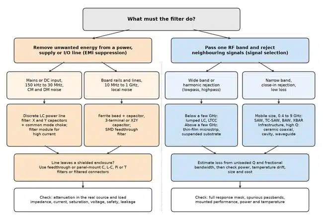
An RF signal filter, by contrast, is normally designed and measured between defined impedances, usually 50 Ω. The specification is a response mask: passband limits and ripple, insertion loss, return loss and rejection at specific frequencies. Table 1 summarises the differences, and Figure 1 shows the decision tree used in this guide.

Aspect	EMI and power-line suppression	RF signal selection
Purpose	Remove broadband noise from power, supply and I/O lines	Pass one band, reject neighbouring signals and harmonics
Typical frequency range	150 kHz to 30 MHz conducted, 30 MHz to 6 GHz radiated	Hundreds of megahertz to millimetre waves
Impedance environment	Low, variable or unknown source and load	Defined, usually 50 Ω
Signal carried	DC, mains or low-frequency signals, often amperes	RF signal, milliwatts to hundreds of watts
Key specifications	Attenuation, rated current and voltage, saturation, safety class, leakage current	Insertion loss, selectivity, bandwidth, return loss, power, temperature drift
Typical technologies	X and Y capacitors, common mode chokes, ferrite beads, feedthrough and 3-terminal capacitors, filtered connectors	Lumped LC, LTCC, microstrip, ceramic coaxial, cavity, waveguide, SAW, BAW

EMI and Power-Line Filter Technologies

Within the EMI branch, the choice is driven by the frequency range of the noise, the line current, the operating voltage and the place where the filter can be installed: at the mains inlet, on the circuit board or in the wall of a shielded enclosure.

Discrete LC Power Line Filters

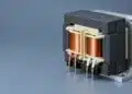
Mains and DC input filters combine X capacitors across the line, Y capacitors from each line to protective earth and a current-compensated common mode choke. In the choke, the load current fluxes of the two windings cancel, so a high-permeability core can provide high common-mode inductance without saturating at the operating current, as explained in toroids and current-compensated chokes. The leakage inductance of the choke adds differential-mode attenuation. These filters cover the conducted range from 150 kHz to 30 MHz and are usually supplied as filter modules for higher currents.

The key selection limits are safety and current rather than RF performance: X and Y capacitors must carry the appropriate safety class, Y capacitance is limited by permissible leakage current, and the choke must be rated for the full current and temperature rise. The calculation of such filters is shown in the AC line filter design and LTspice simulation, and the combination with surge protection in the safe use of varistors and common mode chokes in mains filters.

Ferrite Beads

A ferrite bead is inductive below its crossover frequency, where reactance equals resistance, and predominantly resistive above it. In the resistive region the bead dissipates noise energy as heat, which is the desired operating region for EMI filtering [2]. Typical selection guidance places the impedance peak in the noise band: 30 Ω to 100 Ω for 10 MHz to 50 MHz, 100 Ω to 600 Ω for 50 MHz to 200 MHz and 600 Ω to 1000 Ω for 200 MHz to 1 GHz, as described in selecting a ferrite bead for a buck-boost converter.

DC bias is the main limitation. At 50 % of rated current, the inductance of a bead can fall by up to 90 %, and in one example the impedance at 100 MHz of a 100 Ω, 3 A 0603 bead dropped to 10 Ω [2]. A bead combined with a low-ESR decoupling capacitor also forms an underdamped LC low pass with resonances typically between 0.1 MHz and 10 MHz, which can amplify switching ripple by up to 10 dB unless it is damped [2].

Feedthrough Capacitors and Panel-Mount Filters

In a feedthrough capacitor, the line current passes through the centre conductor, and the capacitor connects to ground around its full circumference. The ground connection therefore has very low inductance, and residual inductance appears in the series path, where it helps filtering, as described in feedthrough capacitor technology and applications. Mounted in the wall of a shielded enclosure, the filter separates the noisy and clean sides and preserves the shielding.

Feedthrough filters are offered as C, L-C, Pi and T sections. Beyond the cutoff frequency, the attenuation slope is about 20 dB per decade for a C section, 40 dB per decade for an L section and 60 dB per decade for a Pi section. Common feedthrough filters provide 40 dB or more at 100 MHz, and the stated maximum for standard C, L and Pi parts is around 70 dB, measured to MIL-STD-220 in a 50 Ω system, as explained in ceramic feedthrough filters.

The configuration is chosen by the impedances on each side. A C filter suits high source and load impedances; in L-C and T filters the inductive element should face the low impedance; a Pi filter suits high impedances on both sides, and a T filter is preferred when both are low [3], [4]. Ferrite elements inside small filters saturate, typically at around 6 A through the pin, and at full load an L-C or Pi filter performs close to a C filter [4].

Three-Terminal, X2Y and SMD Feedthrough Filters

On circuit boards, the inductance of a two-terminal capacitor limits its attenuation at high frequencies. Three-terminal feedthrough chips reduce the ground-return inductance; X2Y capacitors go further by cancelling internal inductance with opposing currents, and because they are used as bypass elements, the load current does not flow through them [4]. One X2Y device can replace several conventional MLCCs in decoupling and balanced-line filtering, as shown in X2Y bypass capacitors and their applications.

Board-mounted filters lose performance above their component resonance, typically from hundreds of megahertz to 1 GHz, and are difficult to make perform like panel-mount parts at these frequencies without a shielding can or a buried-layer board layout [4]. Measured filter characteristics follow theory up to about 100 MHz and diverge significantly above it, with insertion loss falling sharply around 1 GHz because of parasitic elements [5].

Comparing EMI Filter Technologies

Table 2 compares the EMI technologies by the criteria used in this branch. Attenuation values in datasheets are measured in a 50 Ω system at zero load current and room temperature, so real performance is usually lower [4]. Why a filter capacitor performs differently in a real circuit is shown in the introduction to insertion loss and filter capacitor performance.

Technology	Effective range	Attenuation mechanism	Current and saturation	Voltage and safety	Size and cost
X and Y capacitors with common mode choke	150 kHz to 30 MHz conducted	LC voltage divider; CM and DM sections	Choke rated for full current; current compensation avoids CM core saturation	Safety-class capacitors; Y capacitance limited by leakage current	Large, moderate cost; modules for high current
Ferrite bead	About 10 MHz to 1 GHz	Resistive loss above crossover	Impedance falls strongly with DC bias	Low-voltage board lines	Very small, lowest cost
Feedthrough or panel-mount C, L-C, Pi, T	From the cutoff (often about 1 MHz) to the gigahertz range	Low-inductance shunt C plus series L	Centre conductor rating; ferrite saturates at a few amperes	Rated for line or signal voltage	Requires enclosure wall; higher cost per line
3-terminal or X2Y capacitor	Tens of megahertz to the gigahertz range on board	Low-ESL shunt bypass	X2Y not current-limited; 3-terminal limited by electrodes	Low voltage; mains types with safety tests	Very small, low cost
SMD feedthrough or Pi filter	Up to hundreds of megahertz without shielding	Shunt C with bead series elements	Bead saturation	Low voltage	Small, low cost

RF Signal-Selection Filter Technologies

In the RF branch, the main trade-off is between resonator quality, size and cost. Lumped-element filters are the smallest and most economical, ceramic resonator filters have substantially higher unloaded Q and lower loss, and cavity filters provide the lowest loss and highest power handling at the cost of size, weight and price [6]. Higher frequencies increasingly favour distributed technologies such as thin film, suspended substrate stripline and cavities [6].

Why Unloaded Q Sets the Insertion Loss

The resonators of a bandpass filter are characterised by their unloaded quality factor Q_u, which describes the internal conductor, dielectric and radiation losses; the concept is explained in the different approaches to filter Q factor. The dissipative midband loss of a filter with n resonators of equal Q_u can be estimated from the low-pass prototype element values g_k and the fractional bandwidth w = Δf/f₀ with Eq. (1) [7]:

The estimate is approximate, but it explains the selection logic. Loss is inversely proportional to both Q_u and fractional bandwidth, and it grows with the number of resonators needed for steep skirts. The definitions of fractional bandwidth are given in filter bandwidth explained. Table 3 applies Eq. (1) to a five-resonator Chebyshev filter with 0.1 dB ripple, for which the prototype values sum to Σg_k = 7.011.

Unloaded Q	Loss at 1 % bandwidth	Loss at 5 % bandwidth	Representative technology
100	30.4 dB	6.1 dB	Lumped LC with chip inductors
500	6.1 dB	1.2 dB	Microstrip, low-permittivity ceramic resonators
2,000	1.5 dB	0.3 dB	Ceramic coaxial, dielectric and acoustic resonators
5,000	0.6 dB	0.1 dB	Metal cavity, waveguide

A 1 % wide filter at 2 GHz, a 20 MHz passband, is therefore impractical with Q_u = 100 but acceptable with Q_u in the thousands. A 5 % wide filter tolerates much lower Q. This is the main reason why narrowband infrastructure filters use ceramic, cavity or acoustic resonators while broad harmonic filters can use lumped elements or microstrip.

Lumped-Element LC, LTCC and Integrated Passive Filters

Lumped-element filters use discrete or integrated inductors and capacitors. The resonant frequency of each LC resonator follows Eq. (2), although the response of a loaded filter depends on its topology and terminations, as described in lumped-element LC filter design and characteristics:

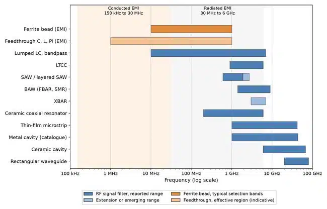
Catalogue capability examples span bandpass centre frequencies of 10 MHz to 7 GHz and lowpass designs up to 22 GHz, with fractional bandwidths from 1 % to more than 100 %. Their resonator Q is limited by the inductors: typical Q is 30 to 100 for wirewound, 20 to 50 for multilayer ceramic and 50 to 200 for thin-film chip inductors, according to RF inductors and LTCC filters. LTCC components cover about 900 MHz to 6 GHz in 0603 to 0805 packages, with bandpass insertion loss of about 2 dB, and practical attenuation usually levels off at 70 dB to 80 dB because of parasitics. LTCC filters are available in sizes down to 0202 with stopband rejection up to 100 dB [8].

Lumped and LTCC filters are the preferred option below a few gigahertz when size and cost dominate, for example in IoT radios, and when the bandwidth is moderate to wide [6].

Microstrip and Thin-Film Planar Filters

Planar filters form their resonators from transmission-line sections whose length is a fraction of the guided wavelength. A quarter-wave resonator on a medium with relative permittivity ε_r, or effective permittivity for microstrip, has the length given by Eq. (3):

At 1 GHz, a quarter wavelength is 75 mm in air and about 45 mm on a microstrip line with an effective permittivity of 2.8. Microstrip filters therefore become practical from about 1 GHz upward. Thin-film filters on ceramic substrates cover 1 GHz to 42 GHz and beyond, with footprint reductions of up to 20 times compared with a typical printed wiring board design when high-permittivity material is used, and lithographic patterning that avoids individual tuning, as described in how microstrip filters work. Connectorised microstrip filters offer 4 % to 40 % fractional bandwidth, insertion loss as low as 0.6 dB and power handling up to 10 W [8].

Distributed filters repeat their response at harmonics of the design frequency. A bandpass filter can have a second passband several times above the intended one, which must be suppressed by an additional lowpass when wideband rejection is required; an example from measured data is shown in filter S-parameters. Microstrip filters suit microwave and millimetre-wave assemblies where moderate Q, repeatability and small planar size are needed; in mmWave phased arrays, single-layer SMT microstrip filters reach more than 50 dB suppression at 26 GHz in a 4 mm × 1.6 mm footprint, as reported in approaching the 5G mmWave filter challenge.

Ceramic Coaxial Resonator Filters

A ceramic coaxial resonator is a metallised high-permittivity ceramic block with a bore. The permittivity shortens the resonator by the factor √ε_r: at 1 GHz, a quarter-wave resonator is about 7.9 mm long in ε_r = 90 ceramic, compared with 75 mm in air, according to Eq. (3). Standard resonators cover about 300 MHz to 6 GHz with ε_r of 21, 37 and 90 and temperature coefficients of resonant frequency within ±10 ppm/K; their Q rises with frequency and resonator size and is determined mainly by the metallisation [9]. Material sets with permittivities from about 5 to 98 are offered, with temperature coefficients below ±5 ppm/K for the lower-permittivity grades [10].

Bandpass filters built from 12 mm and 18 mm resonators cover centre frequencies from 200 MHz to 2.2 GHz with 0.2 % to 30 % fractional bandwidth, and filters with 2 mm to 6 mm resonators cover 1 GHz to 6 GHz with 3 % to 45 % bandwidth, as described in ceramic coaxial resonator filter basics. Catalogue filters reach typical insertion loss of 0.5 dB and power handling up to 20 W [8]. Ceramic filters fill the middle ground between PCB-based filters and larger cavity filters, and cross-coupled topologies add transmission zeros for higher selectivity without much increase in size [6].

Cavity and Waveguide Filters

Cavity filters use air-filled or dielectric-loaded metal resonators with very high unloaded Q, which allows extremely low insertion loss and RF power handling up to hundreds of watts; their drawbacks are size, weight and cost [6]. Catalogue cavity filters reach bandwidths as narrow as 1 %, passbands to 43.5 GHz and stopband rejection above 100 dB [8]. Dielectric resonators used in compact ceramic cavity filters reach Q up to 2,000 from 2 GHz to beyond 40 GHz [11]. Compact ceramic cavity filters span about 6 GHz to 67 GHz with typical insertion loss of 2 dB to 4 dB and 1 % to 5 % bandwidth, while metal-enclosure designs serve transmitters, repeaters, microwave links, radar and satellite links, as covered in cavity resonator filter basics.

According to the same 5G mmWave filter article, rectangular waveguide filters are commonly used from about 20 GHz to 80 GHz, where they combine low loss with high power handling but have centimetre-scale dimensions. Suspended substrate stripline offers an intermediate solution for broadband, high-power applications, with much of the field travelling in air [6].

SAW Filters

Surface acoustic wave filters convert the electrical signal to an acoustic wave with interdigital transducers on a piezoelectric substrate. Because the acoustic velocity is about 75,000 times lower than the speed of light, the wavelength λ at frequency f, given by Eq. (4), is in the micrometre range:

With a surface-wave velocity of 4,022 m/s on 42° Y-X lithium tantalate [12], the acoustic wavelength at 2 GHz is about 2.0 µm, so the electrodes of a standard transducer are about 0.5 µm wide. Above 2 GHz, the transducer electrodes are typically narrower than 1 µm [13], and this lithographic limit sets the practical upper frequency. Standard SAW addresses about 600 MHz to 1.9 GHz, while layered SAW variants such as TF-SAW and IHP-SAW extend the range to about 2.7 GHz [14].

Temperature drift is the main weakness of conventional SAW. Lithium tantalate SAW resonators have a frequency drift of about -38 ppm/K to -60 ppm/K, while layered structures on silicon reach -8 ppm/K and Q of about 4,000 at 2 GHz [15]. Temperature-compensated SAW improves stability at higher cost, and layered SAW costs more again [14]. SAW filters in wafer-level packages occupy less than 1 mm² [13].

BAW, FBAR and XBAR Filters

Bulk acoustic wave filters excite a thickness-mode resonance in a thin piezoelectric film of AlN or ScAlN between two electrodes. The resonant frequency is set by the film thickness rather than by electrode width, so BAW scales to higher frequencies than SAW. The resonator is isolated from the substrate either by a stacked acoustic reflector (SMR) or by an air cavity (FBAR) [14]. Commercial BAW technology covers about 1 GHz to above 8 GHz with Q on the order of 4,000, and the first-order temperature coefficient of AlN resonators is about -25 ppm/K, which can be compensated with SiO₂ layers [15]. The differences between the two acoustic families are compared in the filtering differences between SAW and BAW.

Power handling is a practical limit of all acoustic filters, because power density in a resonator rises with frequency, while BAW handles more power than SAW at high frequencies [15]. In one comparison at equal insertion loss, the temperature rose by 20 °C per watt of transmit power for an SMR-type BAW and by 70 °C per watt for an FBAR [14]. XBAR resonators excite bulk waves in a thin single-crystal lithium niobate membrane with interdigital electrodes and target 3 GHz to 7 GHz with relative bandwidths of 10 % or more [15]. A commercial XBAR filter for 5150 MHz to 7125 MHz has typical insertion loss of 2.2 dB, as reported in the first high-frequency XBAR filter [16].

Comparing RF Filter Technologies

Figure 2 shows the frequency ranges reported for each technology, and Table 4 compares them by the criteria of the RF branch.

Technology	Typical frequency	Fractional bandwidth	Insertion loss and Q	Power	Size	Temperature stability	Relative cost
Lumped LC, LTCC, IPD	10 MHz to about 7 GHz (lowpass higher)	1 % to above 100 %	Inductor Q 20 to 200; LTCC bandpass about 2 dB	Low to moderate	Smallest; LTCC down to 0202	Set by components	Lowest
Thin-film microstrip	1 GHz to 42 GHz and beyond	About 4 % to 40 %	Moderate Q; from 0.6 dB	Up to about 10 W	Millimetres, planar	Substrate-dependent; specified -55 °C to 125 °C	Moderate
Ceramic coaxial resonator	About 0.2 GHz to 6 GHz	0.2 % to 45 %	High Q; from 0.5 dB	Up to about 20 W	Millimetres to centimetres	Resonator drift within about ±15 ppm/K	Moderate
Cavity, waveguide	About 1 GHz to 80 GHz	About 0.5 % to 15 %	Highest Q; lowest loss	Tens to hundreds of watts	Centimetres, heaviest	Mechanically stable designs	Highest
SAW, TC-SAW, layered SAW	About 0.6 GHz to 2.7 GHz	Narrow to moderate	Low loss; Q up to about 4,000 in layered SAW	Limited, falls with frequency	Below 1 mm² in WLP	-38 to -60 ppm/K standard; about -8 ppm/K layered	Low to moderate
BAW (SMR, FBAR), XBAR	About 1.4 GHz to 9 GHz	Narrow to about 10 %	Low loss; Q about 4,000	Better than SAW, still limited	1 mm² to 2 mm² in WLP	About -25 ppm/K uncompensated AlN	Low in volume

Decision Procedure

The procedure below combines both branches into one sequence. Steps 3 to 5 refer to the EMI branch, steps 6 to 8 to the RF branch.

1. Define the job. Write down whether the filter suppresses noise on a power, supply or I/O line or selects an RF band in a signal path.
2. Set the frequency range. For EMI, use the failing frequencies of the emission test or the required immunity range; for RF, use the passband and the frequencies that must be rejected.
3. EMI: separate the noise modes. Common-mode noise is addressed with chokes and Y capacitors, differential-mode noise with X capacitors and series inductance.
4. EMI: choose the location. Mains inlet filters for conducted noise, ferrite beads and low-inductance capacitors on board rails, feedthrough or panel-mount filters where lines leave a shielded enclosure.
5. EMI: check current, voltage and safety. Verify saturation at operating current, voltage and temperature derating of ceramic capacitors, safety classes and leakage current.
6. RF: calculate the fractional bandwidth and required Q. Use the required loss and number of resonators to estimate the minimum unloaded Q.
7. RF: shortlist the technologies. Combine the frequency and Q requirement with the available size: lumped or LTCC at low frequencies, acoustic filters in mobile bands, ceramic, cavity or waveguide filters where Q and power dominate, thin film at microwave and millimetre-wave frequencies.
8. RF: check power and temperature. Compare transmit power, frequency drift over temperature and spurious passbands with the full response mask.
9. Verify in the application. Measure the mounted filter in its real impedances, layout and enclosure.

Selection Checklist

• Application branch: EMI or power-line suppression, or RF signal selection.
• Frequency: noise or passband range, frequencies to be rejected, harmonics and spurious passbands.
• Bandwidth: fractional bandwidth and the definition of the band edges.
• Insertion loss: maximum passband loss for RF; minimum attenuation in the real impedances for EMI.
• Selectivity: rejection at specific frequencies and transition width.
• Power or current: RF power, peak and average, or DC and AC current with saturation behaviour.
• Voltage and safety: working voltage, safety class, leakage current and insulation for line filters.
• Size and mounting: board footprint, panel or enclosure mounting, height and weight.
• Stability: frequency drift over temperature, capacitance change with voltage and temperature.
• Cost and supply: catalogue or custom part, tuning effort and volume.

Conclusion

Passive filter technologies only compete with each other within the same application. On power and I/O lines, the choice between LC power line filters, ferrite beads, feedthrough filters and low-inductance capacitors depends on the noise frequency and mode, the line current and voltage, safety requirements and the installation point, and attenuation must be judged in the real impedances rather than in a 50 Ω test fixture.

In RF signal paths, the required fractional bandwidth and insertion loss define the minimum unloaded Q, and the frequency and available size then narrow the choice: lumped LC and LTCC filters at low frequencies and moderate bandwidths, SAW, BAW and XBAR filters in mobile bands, ceramic coaxial, cavity and waveguide filters where loss and power matter most, and thin-film microstrip filters at microwave and millimetre-wave frequencies. The linked technology articles give the detail needed for the final choice.

FAQ

How to Select a Passive Filter Technology

Further Reading

• Five Key Filter Specifications: the parameters used throughout this guide.
• Filter Shape Factor and Selectivity: how steep skirts are specified.
• Basic Filter Circuits Explained: lowpass, highpass, bandpass and bandstop responses.
• Resonators as Microwave Devices: resonator types behind RF filters.
• To Use or Not to Use a Ferrite Bead in a Power Rail: damping and resonance of bead filters.
• Input Filters for DC/DC Converters: EMI filters at converter inputs.
• How to Pass Conducted Emissions Using Line Filters: conducted emission tests and line filters.
• 3-Phase EMI Filter Design, Simulation, Calculation and Test: power line filters for three-phase systems.

References

1. Fundamentals of EMI Requirements for an Isolated DC/DC Converter, Texas Instruments, white paper SLYY202.
2. J. Eco, A. Limjoco, AN-1368 Ferrite Bead Demystified, Analog Devices, application note.
3. P. Matthews, Insertion Loss and Performance in EMI Filtering, Knowles Precision Devices blog, 2019.
4. S. Hopwood, EMI Filter Hints and Tips, Syfer Technology, 2010.
5. EMI Suppression Filters 3, Guidelines for EMI Suppression, Chapter 6, Murata Manufacturing.
6. Classical RF Filters: Selecting the Right Solution from Lumped Elements to High-Q Cavities, Mini-Circuits, Microwave Journal, October 2026.
7. B. Lake, W. V. Reeder, Notes on the Design of Microstrip and Stripline Bandpass Filters, Royal Aircraft Establishment, Technical Report 74068, 1974.
8. Filter Technologies, Mini-Circuits blog.
9. Coaxial Resonators, product data, Temex Ceramics.
10. Ceramic Resonators, product information, Knowles Precision Devices.
11. P. Matthews, Filter Basics 10: Resonators as Microwave Devices, Knowles Precision Devices blog, 2022.
12. Lithium Tantalate (LiTaO3) Properties, Roditi International.
13. X. Liu et al., A Review of Wafer-Level Packaging Technology for SAW and BAW Filters, Micromachines, vol. 16, no. 3, 320, 2025.
14. RF Filter Technology For Dummies, Qorvo 2nd Special Edition, Wiley/Qorvo, 2022.
15. A. Hagelauer et al., From Microwave Acoustic Filters to Millimeter-Wave Operation and New Applications, IEEE Journal of Microwaves, vol. 3, no. 1, 2023.
16. Murata Releases the World’s First High-Frequency XBAR Filter, Murata Manufacturing, press release, July 2025.
17. Knowles – EPCI premium supplier page, Passive Components Blog.
18. Murata – EPCI premium supplier page, Passive Components Blog.

Article written and technically reviewed in November 2026